Preparation is the key to success in any interview. In this post, we’ll explore crucial Python (NumPy, Pandas, Scikit-learn) interview questions and equip you with strategies to craft impactful answers. Whether you’re a beginner or a pro, these tips will elevate your preparation.
Questions Asked in Python (NumPy, Pandas, Scikit-learn) Interview
Q 1. Explain the difference between NumPy arrays and Python lists.
NumPy arrays and Python lists are both used to store collections of data, but they differ significantly in their functionality and performance. Python lists are general-purpose containers that can hold elements of different data types. NumPy arrays, on the other hand, are designed specifically for numerical operations and are much more efficient for mathematical computations. They are homogeneous, meaning all elements must be of the same data type.
- Data Type Homogeneity: NumPy arrays enforce a single data type for all elements, leading to memory efficiency and faster computations. Python lists can hold elements of varying types.
- Performance: NumPy arrays are optimized for numerical computations using vectorized operations. This means operations are applied to entire arrays at once, rather than element by element, resulting in significant speed improvements compared to looping through Python lists.
- Functionality: NumPy provides a vast library of mathematical and scientific functions that operate directly on arrays, making complex calculations straightforward. Python lists lack this built-in mathematical functionality.
Imagine you’re working with sensor data – thousands of temperature readings. A NumPy array would be the ideal choice because it can efficiently store and process these numerical values. Using Python lists for this task would be significantly slower and less convenient.
import numpy as np
my_array = np.array([1, 2, 3, 4, 5])
my_list = [1, 2, 3, 4, 5]
print(my_array * 2) # efficient element-wise multiplication
print(my_list * 2) # replicates the list, not element-wise multiplication
Q 2. How do you perform element-wise operations in NumPy?
Element-wise operations in NumPy apply an operation to each corresponding element in two or more arrays (or an array and a scalar). This is achieved using standard arithmetic operators like +, -, *, /, //, %, **. NumPy’s vectorized nature handles these operations efficiently without explicit looping.
import numpy as np
arr1 = np.array([1, 2, 3])
arr2 = np.array([4, 5, 6])
print(arr1 + arr2)  # Element-wise addition
print(arr1 * arr2)  # Element-wise multiplication
print(arr1 ** 2) # Element-wise squaring
For instance, imagine calculating the total cost of items given their prices and quantities. If prices are stored in one array and quantities in another, element-wise multiplication immediately gives the total cost for each item.
Q 3. What are broadcasting rules in NumPy?
Broadcasting in NumPy allows arithmetic operations between arrays of different shapes under certain conditions. The smaller array is ‘stretched’ or ‘broadcast’ to match the shape of the larger array before the operation is performed. This avoids explicit reshaping and simplifies code.
The rules for broadcasting are as follows:
- Rule 1: If the arrays have different numbers of dimensions, the shape of the smaller array is padded with leading 1s.
- Rule 2: If the arrays have different sizes in a dimension, one of them must have size 1 in that dimension.
- Rule 3: If both arrays have size 1 in a dimension, then they are compatible.
If these rules are met, broadcasting occurs; otherwise, a ValueError is raised.
import numpy as np
arr1 = np.array([[1, 2, 3], [4, 5, 6]])
arr2 = np.array([10, 20, 30])
print(arr1 + arr2) # Broadcasting arr2 to match arr1's shape
Consider applying a discount rate to a list of product prices. Broadcasting lets you apply the same discount to all prices without explicit looping or reshaping.
Q 4. Describe different ways to create a Pandas DataFrame.
Pandas DataFrames are versatile data structures. You can create them in several ways:
- From a dictionary: Keys become column names, and values (lists or arrays) become column data. This is often the most intuitive method.
- From a list of lists: Each inner list represents a row, and you can specify column names separately.
- From a NumPy array: This is efficient for numerical data. You’ll typically need to specify column names.
- From a CSV file: Pandas’
read_csv()function is powerful for importing data from external files. - From other data sources: Pandas can also read data from Excel files, SQL databases, and more.
import pandas as pd
# From a dictionary
data = {'col1': [1, 2, 3], 'col2': [4, 5, 6]}
df = pd.DataFrame(data)
# From a list of lists
data = [[1, 4], [2, 5], [3, 6]]
df = pd.DataFrame(data, columns=['col1', 'col2'])
Imagine you’re analyzing customer purchase data. You might create a DataFrame from a CSV file containing customer IDs, purchase dates, and amounts, facilitating further analysis.
Q 5. How do you handle missing data in Pandas?
Missing data, often represented as NaN (Not a Number) in Pandas, is a common issue in real-world datasets. Pandas provides several ways to handle it:
- Detection: Use
df.isnull()ordf.isna()to identify missing values.df.notnull()ordf.notna()find non-missing values. - Removal:
dropna()removes rows or columns with missing data. You can specify the axis (rows or columns) and how many missing values trigger removal (e.g., `thresh` parameter). - Imputation: Fill in missing values using
fillna(). You can replace NaNs with a specific value, the mean, median, forward or backward fill, or interpolation methods.
import pandas as pd
df = pd.DataFrame({'A': [1, 2, np.nan], 'B': [4, np.nan, 6]})
print(df.isnull())
print(df.fillna(0)) # Fill with 0
print(df.fillna(method='ffill')) # Forward fill
In a medical dataset, missing blood pressure readings might be imputed using the average blood pressure for patients of similar age and gender.
Q 6. Explain the difference between loc and iloc in Pandas.
Both loc and iloc are used for data selection in Pandas DataFrames, but they differ in how they select rows and columns:
loc: Selects data based on labels (row and column names).iloc: Selects data based on integer positions (indices).
import pandas as pd
df = pd.DataFrame({'A': [1, 2, 3], 'B': [4, 5, 6]}, index=['X', 'Y', 'Z'])
print(df.loc['Y', 'B']) # Selects value at row label 'Y', column label 'B' (5)
print(df.iloc[1, 1]) # Selects value at row index 1, column index 1 (5)
Consider analyzing sales data. If columns are named ‘Region’ and ‘Sales’, loc would be used to select sales from a specific region by name. iloc could be used to extract a block of data based on numerical indices.
Q 7. How do you merge or join DataFrames in Pandas?
Merging and joining DataFrames combine data from multiple sources. The methods differ based on the relationship between the DataFrames:
merge(): Combines DataFrames based on shared columns (keys). It’s similar to SQL joins.join(): Combines DataFrames using their indices. It’s convenient when one DataFrame’s index aligns with another’s column(s).
merge() offers various join types (inner, left, right, outer), controlling which rows are included in the result. Specify the `on` parameter (shared column name) or `left_on` and `right_on` (different column names in each DataFrame).
import pandas as pd
df1 = pd.DataFrame({'key': ['A', 'B', 'C'], 'value1': [1, 2, 3]})
df2 = pd.DataFrame({'key': ['B', 'C', 'D'], 'value2': [4, 5, 6]})
merged_df = pd.merge(df1, df2, on='key', how='inner') # Inner join
Imagine combining customer demographics with their purchase history. You would `merge()` the two DataFrames using a common ‘CustomerID’ column, potentially using a left join to include all customer information even if a purchase isn’t recorded.
Q 8. What are some common data manipulation techniques in Pandas?
Pandas offers a powerful arsenal of tools for data manipulation. Think of it as a Swiss Army knife for your data – capable of handling a wide range of tasks efficiently.
- Data Selection and Filtering: You can select specific columns using
df['column_name']or rows based on conditions using boolean indexing (e.g.,df[df['column_name'] > 10]). This allows you to isolate the data you need for analysis. - Data Cleaning: Pandas makes it easy to handle missing values (using
fillna()), remove duplicates (usingdrop_duplicates()), and replace incorrect data. For example, you can replace missing ages with the average age usingdf['age'].fillna(df['age'].mean()). - Data Transformation: You can easily create new columns based on existing ones (e.g.,
df['new_column'] = df['column1'] + df['column2']), apply functions to entire columns (usingapply()), and change data types (usingastype()). - Data Reshaping: Pandas allows you to reshape your data using functions like
pivot_table()(for creating summary tables),melt()(for converting wide data to long format), andstack()/unstack()(for rearranging hierarchical indices). - Data Joining and Merging: Similar to SQL joins, Pandas allows you to combine data from multiple DataFrames using functions like
merge()andconcat(), providing flexibility in integrating datasets.
Imagine analyzing customer sales data. You might use Pandas to filter for high-value customers, calculate their average purchase amount, and then merge this information with demographic data to identify patterns.
Q 9. Explain the concept of data cleaning and preprocessing.
Data cleaning and preprocessing are crucial steps before applying any machine learning model. It’s like preparing ingredients before cooking – if your ingredients are messy, your dish won’t be good. This involves handling inconsistencies, inaccuracies, and missing information in your dataset to ensure data quality and model accuracy.
- Handling Missing Values: Missing data can be dealt with by imputation (filling in missing values with estimated values like mean, median, or using more advanced techniques like KNN imputation), or by removing rows or columns with excessive missing data. The best approach depends on the nature and amount of missing data.
- Outlier Detection and Treatment: Outliers are extreme values that can skew your results. They can be identified using box plots, scatter plots, or statistical methods (e.g., z-score). Treatment options include removal, transformation (e.g., logarithmic transformation), or capping (replacing outliers with less extreme values).
- Data Transformation: This often involves scaling or normalizing features to ensure that features with larger values don’t dominate the model. Techniques include standardization (z-score normalization) and min-max scaling.
- Encoding Categorical Variables: Machine learning models generally work with numerical data. Categorical features (e.g., colors, genders) need to be converted into numerical representations using techniques like one-hot encoding or label encoding.
For example, in a housing price prediction model, you would clean missing values in features like square footage, and you’d handle outliers in price to build a more reliable model.
Q 10. What are the different types of data structures in Pandas?
Pandas primarily uses two core data structures:
- Series: A one-dimensional labeled array capable of holding any data type (integers, strings, floating point numbers, Python objects, etc.). Think of it as a single column of a spreadsheet.
- DataFrame: A two-dimensional labeled data structure with columns of potentially different types. It’s essentially a table, like a spreadsheet or SQL table, with rows and columns.
A Series is like a single column of data, whereas a DataFrame is a collection of Series, making it suitable for representing tabular data. For instance, you might have a Series representing customer IDs, and another representing their purchase amounts. A DataFrame would then combine these Series to hold all customer data.
Q 11. How do you perform data aggregation and grouping in Pandas?
Data aggregation and grouping in Pandas involves summarizing data based on categories or groups. It’s like organizing your receipts by category (groceries, entertainment, etc.) to get a better understanding of your spending.
The core functions are groupby() and aggregation functions like sum(), mean(), count(), min(), max().
For example, to calculate the average sales per product category:
import pandas as pd data = {'Category': ['A', 'B', 'A', 'C', 'B'], 'Sales': [100, 200, 150, 300, 250]} df = pd.DataFrame(data) average_sales = df.groupby('Category')['Sales'].mean() print(average_sales) This code first groups the data by ‘Category’ and then calculates the mean of ‘Sales’ for each group.
Q 12. What are some common data visualization techniques using Pandas and Matplotlib?
Pandas works seamlessly with Matplotlib to create insightful visualizations. Pandas provides the data, and Matplotlib handles the plotting.
- Histograms: Show the distribution of a single numerical variable.
df['column_name'].hist() - Scatter Plots: Show the relationship between two numerical variables.
df.plot.scatter(x='column1', y='column2') - Bar Charts: Show comparisons between categories.
df.groupby('category')['value'].sum().plot.bar() - Line Charts: Show trends over time.
df.plot.line(x='time', y='value') - Box Plots: Show the distribution of data for different categories, including outliers.
df.boxplot(column='value', by='category')
For example, to visualize the distribution of customer ages, you’d use a histogram. To see the correlation between house size and price, you’d use a scatter plot. These visualizations help quickly understand data patterns.
Q 13. What is Scikit-learn, and what are its core components?
Scikit-learn (sklearn) is a powerful Python library for machine learning. It’s like a toolbox filled with pre-built tools for various machine learning tasks. It offers a consistent interface and extensive documentation, making it easy to use.
Core components include:
- Estimators: These are models that learn patterns from data. Examples include linear regression, support vector machines, decision trees, and random forests. They have methods like
fit()(for training) andpredict()(for making predictions). - Transformers: Used for preprocessing and feature extraction. Examples include scaling, encoding, and dimensionality reduction techniques. They have methods like
fit_transform(). - Model Selection: Tools for evaluating models (e.g., cross-validation) and selecting the best one. This includes tools for hyperparameter tuning (e.g., GridSearchCV).
Think of it as a well-organized toolbox where each tool (estimator, transformer) is designed for a specific task. You can mix and match the tools to create your custom machine learning pipeline.
Q 14. Explain different types of machine learning models in Scikit-learn.
Scikit-learn provides a wide variety of machine learning models, categorized broadly as:
- Supervised Learning: Models that learn from labeled data (data with known outputs).
- Regression: Predicting continuous values (e.g., house prices). Examples include Linear Regression, Support Vector Regression, Decision Tree Regression.
- Classification: Predicting categorical values (e.g., spam/not spam). Examples include Logistic Regression, Support Vector Machines, Decision Trees, Random Forests, Naive Bayes.
- Unsupervised Learning: Models that learn from unlabeled data (data without known outputs).
- Clustering: Grouping similar data points together. Examples include K-Means, DBSCAN.
- Dimensionality Reduction: Reducing the number of features while preserving important information. Examples include Principal Component Analysis (PCA), t-SNE.
- Model Evaluation: Assessing model performance using metrics such as accuracy, precision, recall, F1-score, and AUC (Area Under the Curve).
The choice of model depends on the specific problem, the type of data, and the desired outcome. For example, you’d use a regression model to predict house prices and a classification model to detect fraudulent transactions.
Q 15. How do you perform data splitting for model training and testing?
Data splitting is crucial for evaluating the generalization performance of a machine learning model. We avoid training and testing on the same data to prevent overfitting, where the model memorizes the training data instead of learning general patterns. The most common approach is to split the data into two sets: a training set and a testing set.
The training set is used to train the model, allowing it to learn the relationships between features and target variables. The testing set, unseen during training, is used to evaluate the model’s performance on new, unseen data, giving a realistic estimate of its generalization ability. A typical split is 80% for training and 20% for testing, but this can vary depending on the dataset size and complexity. Scikit-learn provides a convenient function for this:
from sklearn.model_selection import train_test_split
X_train, X_test, y_train, y_test = train_test_split(X, y, test_size=0.2, random_state=42)
Here, X represents the features and y represents the target variable. test_size=0.2 specifies a 20% test split, and random_state=42 ensures reproducibility by setting a seed for the random number generator.
For larger datasets, consider using stratified sampling to maintain class proportions in both the training and testing sets, especially for imbalanced datasets. This ensures a fair evaluation of the model’s performance across different classes.
Career Expert Tips:
- Ace those interviews! Prepare effectively by reviewing the Top 50 Most Common Interview Questions on ResumeGemini.
- Navigate your job search with confidence! Explore a wide range of Career Tips on ResumeGemini. Learn about common challenges and recommendations to overcome them.
- Craft the perfect resume! Master the Art of Resume Writing with ResumeGemini’s guide. Showcase your unique qualifications and achievements effectively.
- Don’t miss out on holiday savings! Build your dream resume with ResumeGemini’s ATS optimized templates.
Q 16. What are the common evaluation metrics for classification and regression problems?
Evaluation metrics quantify the performance of a machine learning model. They differ based on whether the problem is classification or regression.
- Classification Metrics: These assess the model’s ability to correctly classify instances into different categories.
- Accuracy: The ratio of correctly classified instances to the total number of instances. Simple but can be misleading with imbalanced classes.
- Precision: The proportion of correctly predicted positive instances among all instances predicted as positive. Answers ‘Of all the instances predicted as positive, what proportion was actually positive?’
- Recall (Sensitivity): The proportion of correctly predicted positive instances among all actual positive instances. Answers ‘Of all the actual positive instances, what proportion did we correctly predict?’
- F1-score: The harmonic mean of precision and recall, providing a balanced measure. Useful when both precision and recall are important.
- AUC-ROC (Area Under the Receiver Operating Characteristic Curve): Measures the model’s ability to distinguish between classes across different thresholds. A higher AUC indicates better performance.
- Regression Metrics: These evaluate how well the model predicts continuous values.
- Mean Squared Error (MSE): The average of the squared differences between predicted and actual values. Sensitive to outliers.
- Root Mean Squared Error (RMSE): The square root of MSE, providing a value in the same units as the target variable. Easier to interpret than MSE.
- Mean Absolute Error (MAE): The average of the absolute differences between predicted and actual values. Less sensitive to outliers than MSE.
- R-squared (R2): Represents the proportion of variance in the target variable explained by the model. Ranges from 0 to 1, with higher values indicating better fit.
Choosing the right metric depends heavily on the specific problem and business objectives. For instance, in fraud detection (a classification problem), recall might be prioritized over precision to minimize false negatives (missed fraudulent transactions).
Q 17. How do you handle overfitting and underfitting in machine learning models?
Overfitting and underfitting are common challenges in machine learning. They represent opposite ends of the model’s ability to generalize to unseen data.
- Overfitting: Occurs when a model learns the training data too well, including noise and outliers. This leads to excellent performance on the training set but poor performance on the testing set. Think of it as memorizing the answers instead of understanding the concepts.
- Underfitting: Occurs when a model is too simple to capture the underlying patterns in the data. This results in poor performance on both the training and testing sets. Think of it as having a too-shallow understanding of the material.
Here’s how to address these issues:
- Overfitting:
- Reduce model complexity: Use simpler models with fewer parameters (e.g., linear regression instead of a high-degree polynomial).
- Regularization: Add penalty terms to the model’s loss function to discourage large weights (discussed in the next question).
- Cross-validation: Use techniques like k-fold cross-validation to get a more robust estimate of model performance.
- Increase training data: More data can help the model generalize better.
- Feature selection/engineering: Remove irrelevant or redundant features.
- Underfitting:
- Increase model complexity: Use more complex models with more parameters (e.g., add more layers to a neural network).
- Add more features: Include additional features that might capture relevant information.
- Improve feature engineering: Create new features that better represent the underlying patterns.
Identifying the problem is key. If the training error is low but the testing error is high, it’s overfitting. If both are high, it’s underfitting.
Q 18. Explain the concept of regularization in machine learning.
Regularization is a technique used to prevent overfitting by adding a penalty term to the model’s loss function. This penalty discourages the model from learning overly complex relationships and assigning excessively large weights to individual features. It essentially ‘shrinks’ the weights towards zero.
The most common types of regularization are:
- L1 Regularization (LASSO): Adds a penalty term proportional to the absolute values of the weights. This encourages sparsity, meaning some weights become exactly zero, effectively performing feature selection.
- L2 Regularization (Ridge): Adds a penalty term proportional to the square of the weights. This shrinks the weights towards zero but doesn’t force them to be exactly zero.
In scikit-learn, you can easily incorporate regularization into linear models:
from sklearn.linear_model import Ridge, Lasso
ridge_model = Ridge(alpha=1.0) # alpha controls the strength of regularization
lasso_model = Lasso(alpha=1.0)
The alpha parameter controls the strength of regularization. A larger alpha means stronger regularization.
The choice between L1 and L2 depends on the problem. L1 is preferred when feature selection is desired, while L2 is often preferred for its stability and less sensitivity to outliers.
Q 19. Describe different techniques for feature scaling and selection.
Feature scaling and selection are crucial preprocessing steps that significantly impact model performance.
Feature Scaling: This involves transforming features to a similar scale to prevent features with larger values from dominating the model. Common techniques include:
- Standardization (Z-score normalization): Centers the data around zero with a unit standard deviation.
(x - mean) / standard deviation - Min-Max scaling: Scales features to a specific range, typically [0, 1].
(x - min) / (max - min)
Scikit-learn provides functions for these:
from sklearn.preprocessing import StandardScaler, MinMaxScaler
scaler = StandardScaler()
X_scaled = scaler.fit_transform(X)
Feature Selection: This aims to identify the most relevant features, removing irrelevant or redundant ones that can negatively impact model performance. Techniques include:
- Filter methods: Rank features based on statistical measures (e.g., correlation with the target variable, chi-squared test). Simple and computationally efficient.
- Wrapper methods: Evaluate subsets of features using a model’s performance (e.g., recursive feature elimination). More computationally expensive but potentially more accurate.
- Embedded methods: Incorporate feature selection into the model’s training process (e.g., L1 regularization, tree-based models). Efficient and often effective.
The choice of scaling and selection techniques depends on the dataset and the model used. Experimentation is often necessary to determine the optimal approach.
Q 20. How do you perform hyperparameter tuning for machine learning models?
Hyperparameter tuning involves finding the optimal settings for the parameters of a machine learning model that are not learned during training. These parameters control the model’s learning process, such as the learning rate in gradient descent or the number of trees in a random forest.
Common techniques include:
- Grid Search: Exhaustively searches a predefined set of hyperparameter values. Simple but can be computationally expensive for large search spaces.
- Random Search: Randomly samples hyperparameter values from a specified distribution. Often more efficient than grid search, especially for high-dimensional search spaces.
- Bayesian Optimization: Uses a probabilistic model to guide the search, focusing on promising regions of the hyperparameter space. More computationally expensive but often finds good solutions faster than random search.
Scikit-learn provides tools for these:
from sklearn.model_selection import GridSearchCV, RandomizedSearchCV
param_grid = {'n_estimators': [100, 200, 300], 'max_depth': [None, 10, 20]}
grid_search = GridSearchCV(model, param_grid, cv=5)
grid_search.fit(X_train, y_train)
This code performs a grid search for a model using 5-fold cross-validation. The best hyperparameter combination is then selected based on the cross-validated performance.
Q 21. What is cross-validation, and why is it important?
Cross-validation is a resampling technique used to evaluate a model’s performance and reduce the risk of overfitting. It involves splitting the data into multiple folds (subsets), training the model on some folds, and evaluating it on the remaining folds. This process is repeated multiple times, with different folds used for training and testing each time.
The most common type is k-fold cross-validation, where the data is split into k equal-sized folds. The model is trained k times, each time using k-1 folds for training and one fold for testing. The performance metrics are then averaged across all k iterations. A common value for k is 5 or 10.
Why is it important?
- More robust performance estimation: Provides a more reliable estimate of the model’s generalization performance compared to a single train-test split.
- Reduced overfitting risk: By using multiple training and testing sets, it helps identify models that overfit to specific subsets of the data.
- Improved hyperparameter tuning: Can be used to select the best hyperparameter settings for a model by evaluating performance across different folds.
Scikit-learn makes cross-validation easy:
from sklearn.model_selection import cross_val_score
scores = cross_val_score(model, X, y, cv=5)
This code performs 5-fold cross-validation and returns an array of scores for each fold. The average of these scores provides a robust performance estimate.
Q 22. Explain the difference between supervised and unsupervised learning.
Supervised and unsupervised learning are two major categories of machine learning algorithms, distinguished by the presence or absence of labeled data. Think of it like this: supervised learning is like having a teacher who provides you with the correct answers (labels) for each example, while unsupervised learning is like exploring a vast dataset without a teacher, trying to find patterns on your own.
Supervised Learning: Algorithms learn from a labeled dataset, where each data point is associated with a known outcome (target variable). The goal is to learn a mapping from inputs to outputs, allowing the model to predict the output for new, unseen inputs. Examples include linear regression (predicting a continuous value), logistic regression (predicting a binary outcome), and decision trees (predicting categorical outcomes).
Unsupervised Learning: Algorithms learn from an unlabeled dataset, where no target variable is provided. The goal is to discover hidden patterns, structures, or relationships within the data. Examples include clustering (grouping similar data points together), dimensionality reduction (reducing the number of variables while preserving important information), and anomaly detection (identifying unusual data points).
Q 23. How do you implement linear regression using Scikit-learn?
Linear regression is a supervised learning algorithm used to model the relationship between a dependent variable and one or more independent variables. The goal is to find the best-fitting straight line (or hyperplane in multiple dimensions) that minimizes the difference between the predicted and actual values of the dependent variable.
Here’s how to implement it using Scikit-learn:
from sklearn.linear_model import LinearRegression
from sklearn.model_selection import train_test_split

# Sample data
X = [[1], [2], [3]]  # Independent variable
y = [2, 4, 5]      # Dependent variable

# Split data into training and testing sets
X_train, X_test, y_train, y_test = train_test_split(X, y, test_size=0.2, random_state=42)

# Create and train the model
model = LinearRegression()
model.fit(X_train, y_train)

# Make predictions
y_pred = model.predict(X_test)

# Evaluate the model (e.g., using R-squared)
r2 = model.score(X_test, y_test)
print(f'R-squared: {r2}')
This code snippet shows a basic example. In real-world scenarios, you would likely need to preprocess your data (handle missing values, scale features, etc.) and potentially use more sophisticated techniques for model evaluation and selection.
Q 24. How do you implement logistic regression using Scikit-learn?
Logistic regression is a supervised learning algorithm used for classification problems, where the dependent variable is categorical (often binary, i.e., 0 or 1). Unlike linear regression which predicts a continuous value, logistic regression predicts the probability of an instance belonging to a particular class. This probability is then converted to a class label using a threshold (typically 0.5).
Here’s how to implement it using Scikit-learn:
from sklearn.linear_model import LogisticRegression
from sklearn.model_selection import train_test_split

# Sample data
X = [[1, 2], [2, 3], [3, 1], [4, 3]]
y = [0, 1, 0, 1]

# Split data into training and testing sets
X_train, X_test, y_train, y_test = train_test_split(X, y, test_size=0.2, random_state=42)

# Create and train the model
model = LogisticRegression()
model.fit(X_train, y_train)

# Make predictions
y_pred = model.predict(X_test)

# Evaluate the model (e.g., using accuracy)
accuracy = model.score(X_test, y_test)
print(f'Accuracy: {accuracy}')
Similar to linear regression, data preprocessing is crucial for optimal performance. Metrics like precision, recall, F1-score, and AUC are often used to evaluate logistic regression models, offering a more comprehensive picture than just accuracy.
Q 25. How do you perform decision tree classification using Scikit-learn?
Decision tree classification is a supervised learning algorithm that builds a tree-like model to classify data points. Each internal node represents a feature, each branch represents a decision rule, and each leaf node represents an outcome. The algorithm recursively partitions the data based on the feature that best separates the classes.
Here’s how to implement it using Scikit-learn:
from sklearn.tree import DecisionTreeClassifier
from sklearn.model_selection import train_test_split

# Sample data (same as logistic regression example)
X = [[1, 2], [2, 3], [3, 1], [4, 3]]
y = [0, 1, 0, 1]

# Split data
X_train, X_test, y_train, y_test = train_test_split(X, y, test_size=0.2, random_state=42)

# Create and train the model
model = DecisionTreeClassifier()
model.fit(X_train, y_train)

# Make predictions
y_pred = model.predict(X_test)

# Evaluate the model
accuracy = model.score(X_test, y_test)
print(f'Accuracy: {accuracy}')
Decision trees are prone to overfitting (performing well on training data but poorly on unseen data). Techniques like pruning and ensemble methods (e.g., Random Forest) can mitigate this.
Q 26. How do you perform K-means clustering using Scikit-learn?
K-means clustering is an unsupervised learning algorithm that partitions data points into k clusters, where k is a predefined number. The algorithm aims to minimize the sum of squared distances between each data point and the centroid (mean) of its assigned cluster. Imagine you’re sorting marbles of different colors into separate containers – each container represents a cluster, and the algorithm tries to put marbles of similar colors together.
Here’s how to implement it using Scikit-learn:
from sklearn.cluster import KMeans

# Sample data
X = [[1, 2], [1, 4], [1, 0], [10, 2], [10, 4], [10, 0]]

# Choose the number of clusters (k)
k = 2

# Create and train the model
kmeans = KMeans(n_clusters=k, random_state=42)
kmeans.fit(X)

# Get cluster labels for each data point
labels = kmeans.labels_
print(f'Cluster Labels: {labels}')

# Get cluster centroids
centroids = kmeans.cluster_centers_
print(f'Centroids: {centroids}')
Choosing the optimal number of clusters (k) is a crucial step and often requires techniques like the elbow method or silhouette analysis.
Q 27. How do you evaluate the performance of a clustering model?
Evaluating the performance of a clustering model is more challenging than in supervised learning because there’s no ground truth (no pre-assigned labels). We rely on evaluating the inherent structure and quality of the clusters formed.
Common metrics include:
Silhouette Score: Measures how similar a data point is to its own cluster compared to other clusters. A higher silhouette score indicates better-defined clusters.
Davies-Bouldin Index: Measures the average similarity between each cluster and its most similar cluster. A lower Davies-Bouldin index suggests better-separated clusters.
Calinski-Harabasz Index (Variance Ratio Criterion): Measures the ratio of between-cluster dispersion and within-cluster dispersion. A higher score indicates better clustering.
Visual inspection of the clusters (e.g., using scatter plots) is also important to gain insights into the model’s performance. The choice of evaluation metric depends on the specific application and the desired properties of the clusters.
Q 28. Explain the concept of dimensionality reduction.
Dimensionality reduction is the process of reducing the number of variables (features) in a dataset while retaining as much important information as possible. High-dimensional data can be challenging to work with due to the curse of dimensionality (increased computational cost and potential overfitting). Dimensionality reduction simplifies the data, making it easier to visualize, analyze, and build models.
Techniques include:
Principal Component Analysis (PCA): A linear transformation that projects the data onto a lower-dimensional subspace while maximizing variance. Think of it as finding the most important axes of variation in your data.
t-distributed Stochastic Neighbor Embedding (t-SNE): A non-linear technique that emphasizes local neighborhood structures in the data. It’s particularly useful for visualizing high-dimensional data in lower dimensions (e.g., 2D or 3D).
Feature Selection: Techniques that select a subset of the original features based on their importance or relevance to the target variable (in supervised learning). Methods include filter methods (e.g., correlation analysis), wrapper methods (e.g., recursive feature elimination), and embedded methods (e.g., L1 regularization).
The choice of technique depends on the specific dataset and the goals of the analysis. PCA is widely used for its simplicity and efficiency, while t-SNE is better suited for visualization. Feature selection is often preferred when interpretability is crucial.
Key Topics to Learn for Python (NumPy, Pandas, Scikit-learn) Interview
- NumPy Fundamentals: Arrays, array manipulation (slicing, indexing, reshaping), broadcasting, vectorized operations. Understanding these is crucial for efficient data handling.
- NumPy Linear Algebra: Dot products, matrix operations, eigenvalues and eigenvectors. These concepts underpin many machine learning algorithms.
- Pandas Data Structures: Series and DataFrames, data cleaning (handling missing values, duplicates), data manipulation (filtering, sorting, grouping), data merging and joining. Mastering Pandas is essential for data wrangling.
- Pandas Data Analysis: Descriptive statistics, data aggregation, working with time series data. This demonstrates your ability to extract insights from data.
- Scikit-learn Models: Linear Regression, Logistic Regression, Support Vector Machines (SVMs), Decision Trees, Random Forests. Focus on understanding the underlying principles and practical applications of each model.
- Scikit-learn Model Evaluation: Metrics (accuracy, precision, recall, F1-score, AUC), cross-validation techniques. Knowing how to evaluate model performance is crucial for effective machine learning.
- Data Preprocessing: Feature scaling (standardization, normalization), handling categorical variables (one-hot encoding), feature selection. Clean data is the foundation of successful models.
- Model Selection and Tuning: Hyperparameter tuning using techniques like grid search and cross-validation. This showcases your ability to optimize model performance.
- Python Proficiency: Object-oriented programming principles, working with functions and classes, exception handling. Solid Python skills are fundamental.
- Problem-Solving Approach: Practice breaking down complex problems into smaller, manageable parts. Demonstrate your ability to think critically and logically.
Next Steps
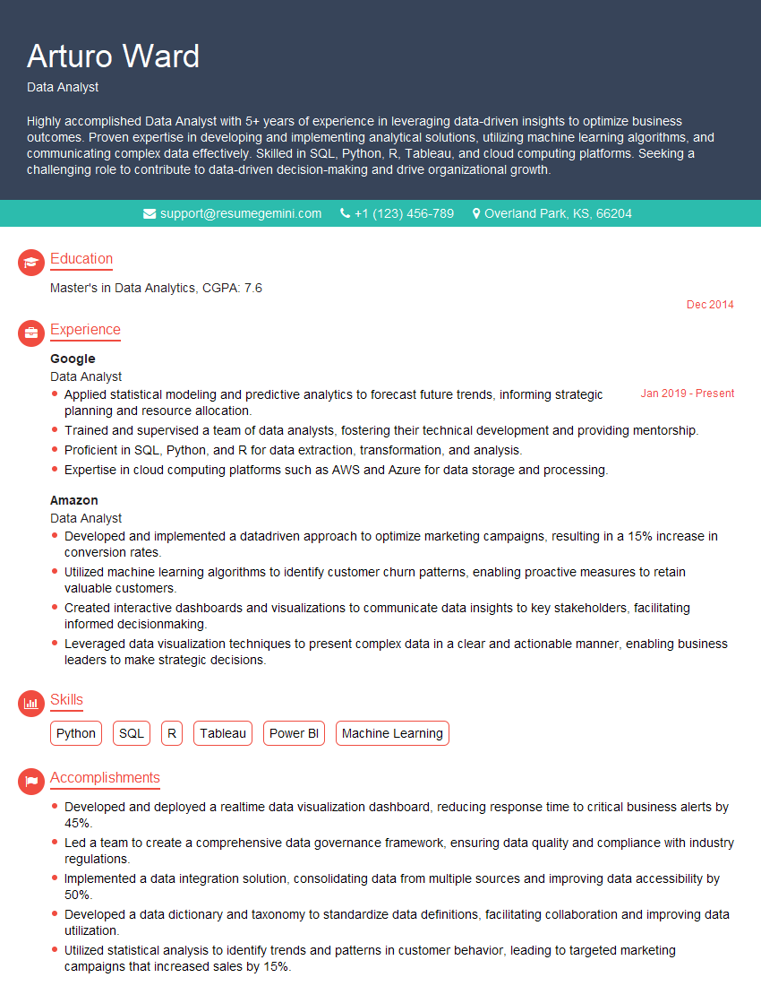
Mastering Python, particularly NumPy, Pandas, and Scikit-learn, is vital for a successful career in data science and machine learning. These libraries are industry standards, and proficiency in them significantly boosts your job prospects. To maximize your chances, crafting a strong, ATS-friendly resume is essential. ResumeGemini is a trusted resource to help you build a professional and impactful resume that highlights your skills effectively. Examples of resumes tailored to showcase expertise in Python, NumPy, Pandas, and Scikit-learn are available to guide you.
Explore more articles
Users Rating of Our Blogs
Share Your Experience
We value your feedback! Please rate our content and share your thoughts (optional).
What Readers Say About Our Blog
This was kind of a unique content I found around the specialized skills. Very helpful questions and good detailed answers.
Very Helpful blog, thank you Interviewgemini team.
