Feeling uncertain about what to expect in your upcoming interview? We’ve got you covered! This blog highlights the most important AMOS (Structural Equation Modeling Software) interview questions and provides actionable advice to help you stand out as the ideal candidate. Let’s pave the way for your success.
Questions Asked in AMOS (Structural Equation Modeling Software) Interview
Q 1. Explain the difference between mediation and moderation in SEM.
In Structural Equation Modeling (SEM), mediation and moderation represent distinct ways a third variable influences the relationship between two other variables. Think of it like this: mediation explains why a relationship exists, while moderation explains when or under what conditions a relationship exists.
Mediation: A mediator variable sits between two other variables, explaining the mechanism through which one variable affects another. For example, let’s say we’re studying the relationship between job stress (X) and burnout (Y). A mediating variable could be emotional exhaustion (M). Job stress (X) leads to emotional exhaustion (M), which in turn leads to burnout (Y). The mediator explains the pathway: stress doesn’t directly cause burnout; rather, it causes exhaustion, which then causes burnout.
Moderation: A moderator variable influences the strength or direction of the relationship between two other variables. Using the same example, let’s say social support (Z) is a moderator. The relationship between job stress (X) and burnout (Y) might be stronger for individuals with low social support and weaker for those with high social support. The moderator changes the effect; the impact of stress on burnout depends on the level of social support.
In AMOS, you test mediation by examining indirect effects (the effect of X on Y through M) and direct effects (the effect of X on Y without M). Moderation is tested by including interaction terms (e.g., X * Z) in the model and assessing their significance.
Q 2. Describe the assumptions of structural equation modeling.
SEM rests on several key assumptions. Violating these assumptions can lead to biased or inaccurate results. Let’s examine them:
- Multivariate normality: The data should be approximately normally distributed across all variables. While minor deviations are often tolerable, severe departures can affect the accuracy of parameter estimates and significance tests. AMOS offers robust estimators to mitigate this concern in cases of non-normality.
- Linearity: The relationships between variables should be linear. Non-linear relationships require transformations or different modeling techniques. Scatterplots and residual analysis can help detect non-linearity.
- No multicollinearity: High correlations between predictor variables can lead to unstable parameter estimates. This is assessed through correlation matrices and variance inflation factors (VIFs). Techniques like principal component analysis could be used to address.
- Correct model specification: The model should accurately reflect the hypothesized relationships between variables. Incorrect model specification leads to biased results. Theory-driven model building and model modification indices can assist in refinement.
- Sufficient sample size: A sufficiently large sample size is crucial for reliable parameter estimates and statistical power. The required sample size depends on the model complexity and the number of parameters estimated. Rules of thumb exist but depend on your specific context, often involving power analyses.
- Random sampling: The data should be obtained through a random sampling method to ensure the results generalize to the population of interest.
Q 3. How do you assess model fit in AMOS?
Assessing model fit in AMOS involves examining multiple fit indices to gain a comprehensive understanding of how well the model represents the observed data. AMOS provides a wealth of fit indices that should be used in combination, not in isolation. No single index perfectly determines model fit. Think of it as a medical diagnosis – you need multiple tests for a clear picture.
The process generally involves:
- Examining overall fit indices: AMOS provides indices such as χ² (chi-square), Comparative Fit Index (CFI), Tucker-Lewis Index (TLI), Root Mean Square Error of Approximation (RMSEA), and Standardized Root Mean Square Residual (SRMR). These provide an overall assessment of how well the model fits the data.
- Inspecting modification indices: These indices suggest potential model modifications to improve fit. However, using these indices excessively can lead to overfitting. Carefully consider theoretical justification before making changes.
- Evaluating standardized residuals and modification indices: Examining these helps detect potential problems with the model or data. Large residuals indicate discrepancies between the model’s predictions and the observed data.
- Visual inspection of path diagrams: AMOS provides a clear visualization of the model, allowing for an intuitive understanding of parameter estimates and relationships. You are looking for estimates that make sense in the context of your theory.
Q 4. What are the different types of fit indices and how do you interpret them?
AMOS offers a variety of fit indices, each with its own strengths and weaknesses. It’s crucial to interpret these indices together, rather than relying solely on a single one.
- χ² (Chi-square): A traditional test of model fit. A non-significant χ² indicates a good fit, but it’s sensitive to sample size (large samples make it more likely to reject a good model). Hence it’s best combined with other indices.
- CFI (Comparative Fit Index): Compares the fit of the model to a baseline model (usually an independence model). Values above 0.95 generally indicate a good fit.
- TLI (Tucker-Lewis Index): Similar to CFI; values above 0.95 suggest a good fit.
- RMSEA (Root Mean Square Error of Approximation): Estimates the discrepancy between the model and the population covariance matrix. Values below 0.05 indicate a close fit, values between 0.05 and 0.08 suggest a reasonable fit, and higher values suggest a poor fit. It’s important to look at the confidence intervals.
- SRMR (Standardized Root Mean Square Residual): Indicates the average standardized residual. Values below 0.08 are usually considered acceptable.
Interpretation: No single ‘magic number’ exists. Consider the overall pattern of indices. For example, a good-fitting model typically shows high CFI and TLI values (>0.95), low RMSEA values (<0.05), and low SRMR values (<0.08).
Q 5. Explain the concept of identification in SEM.
Model identification in SEM refers to whether the model has a unique solution for its parameters. An identified model has only one set of parameter estimates that perfectly reproduce the observed covariance matrix, whereas an under-identified model has multiple possible solutions, and an over-identified model has more restrictions than needed, leading to potential problems.
Rules of identification: Determining identification involves checking the number of observed and unobserved variables, and the number of parameters to estimate. A simple rule of thumb (but not always sufficient) is that the number of unique elements in the observed covariance matrix (p(p+1)/2, where p is the number of observed variables) must be greater than or equal to the number of parameters to estimate in the model. AMOS provides warnings if the model is under-identified. This ensures that the solution provided is sensible and not an artifact of the estimation process.
Under-identification often results from a poorly specified model or a lack of sufficient information to estimate the parameters uniquely. Over-identification indicates that some parameters may be redundant or that there is more information available than necessary.
Q 6. How do you handle missing data in SEM?
Handling missing data is a crucial aspect of SEM. Ignoring missing data can bias the results. AMOS offers several approaches:
- Listwise deletion: This simple method excludes any cases with missing data. However, this can lead to substantial loss of data, especially with multiple variables and can introduce bias if data is not Missing Completely at Random (MCAR).
- Pairwise deletion: This uses all available data for each pair of variables when computing the covariance matrix. This can lead to inconsistencies if the missing data mechanism is not MCAR.
- Full Information Maximum Likelihood (FIML): This sophisticated method is generally preferred. It uses all available information and makes assumptions about the missing data pattern (e.g., MCAR or Missing at Random (MAR)). It’s generally more efficient and less biased than listwise or pairwise deletion, especially if your missing data mechanism is MAR. AMOS implements FIML efficiently, maximizing your sample size and minimizing bias.
- Imputation Methods: Techniques like multiple imputation generate plausible values for missing data. This adds complexity, but can be useful in certain circumstances.
The choice of method depends on the nature and amount of missing data, as well as the assumptions one is willing to make about the data.
Q 7. What are the different estimation methods used in AMOS?
AMOS provides various estimation methods, each with specific advantages and disadvantages:
- Maximum Likelihood (ML): The most common estimation method. It assumes multivariate normality. It’s efficient and generally provides good results when the normality assumption is met.
- Generalized Least Squares (GLS): A robust method less sensitive to deviations from multivariate normality than ML. If normality assumption is violated or sample size is small, GLS could be preferred.
- Weighted Least Squares (WLS): Another robust method, particularly useful when the data are non-normal and the sample size is small.
- Robust Maximum Likelihood (MLR): Provides standard errors and chi-square statistics that are adjusted for non-normality. This is a popular choice when normality is in question, as it addresses the sensitivity of ML to non-normality.
The choice of estimation method depends on the characteristics of the data and the research question. If you suspect non-normality or have a smaller sample size, considering robust methods like GLS, WLS or MLR is highly recommended. AMOS conveniently provides these options, facilitating informed decisions based on your data properties.
Q 8. Compare and contrast Maximum Likelihood and Weighted Least Squares estimation.
Maximum Likelihood (ML) and Weighted Least Squares (WLS) are two common estimation methods in AMOS for Structural Equation Modeling (SEM). Both aim to find the parameter estimates that best fit the observed data to the hypothesized model, but they differ in their assumptions and how they handle data.
- Maximum Likelihood (ML): ML assumes your data is multivariate normal. It maximizes the likelihood of observing the sample data given the model parameters. It’s efficient and yields accurate results when the normality assumption holds. However, it can be sensitive to violations of this assumption, especially with smaller sample sizes or non-normal data.
- Weighted Least Squares (WLS): WLS is a robust alternative that doesn’t assume multivariate normality. It minimizes a weighted sum of squared differences between the observed and implied covariance matrices. This makes it more resistant to violations of normality. However, it generally requires larger sample sizes than ML for accurate results. Furthermore, diagonally weighted least squares (DWLS) is a variation of WLS often preferred as it only requires the observed covariance matrix and not the full sample data, making it more computationally efficient for larger datasets.
In short: Choose ML if your data is approximately multivariate normal and you have a reasonable sample size. Opt for WLS (or DWLS) if you have concerns about normality or if your data violates this assumption significantly.
Q 9. How do you assess the reliability and validity of your measures in AMOS?
Assessing reliability and validity is crucial in SEM. In AMOS, we use several techniques:
- Reliability: This refers to the consistency of your measures. For observed variables, we often use Cronbach’s alpha (available through AMOS’s output or by pre-processing in other statistical software). A Cronbach’s alpha above 0.7 is generally considered acceptable, indicating good internal consistency. For latent variables, we look at the composite reliability (CR). CR values above 0.7 also suggest good reliability.
- Validity: This assesses whether your measures actually capture the intended constructs. Several approaches are used:
- Convergent Validity: Do indicators of the same latent variable correlate highly? Examine factor loadings (standardized estimates) in AMOS; high loadings (e.g., >0.7) suggest good convergent validity.
- Discriminant Validity: Do indicators of different latent variables correlate less highly than indicators of the same latent variable? Examine the correlation between latent variables – they should be significantly lower than the average variance extracted (AVE) for each of the involved constructs.
- Content Validity: Does the measure adequately cover all aspects of the construct? This is evaluated qualitatively based on expert judgment before the analysis.
AMOS provides the necessary statistics for assessing these aspects, allowing for a comprehensive evaluation of the measurement model before analyzing the structural model.
Q 10. Explain the concept of factor analysis and its role in SEM.
Factor analysis is a statistical method used to identify underlying latent variables (factors) that explain the correlations among a set of observed variables. In SEM, it plays a crucial role in assessing the measurement model, which is the part of the model that describes how latent variables relate to observed variables.
Think of it like this: you have many individual pieces of data (observed variables) and factor analysis helps you group them into meaningful clusters (latent variables) based on their relationships. For example, several questions on a survey might all measure ‘job satisfaction’. Factor analysis can identify this latent variable ‘job satisfaction’ and how strongly each question contributes to this underlying construct.
In AMOS, you can perform confirmatory factor analysis (CFA), which tests a pre-specified model of how the observed variables relate to the latent variables. This ensures that your measurement model adequately reflects the relationships before moving to the structural model analysis.
Q 11. How do you specify a latent variable in AMOS?
Specifying a latent variable in AMOS is done graphically using the drawing tools. You don’t directly enter data for a latent variable; instead, you define it by its relationships with observed variables (indicators).
1. **Create an oval shape:** This represents your latent variable. Label it appropriately (e.g., ‘Job Satisfaction’).
2. **Create rectangles:** These represent your observed variables (e.g., specific survey questions about job satisfaction).
3. **Draw single-headed arrows:** These link the latent variable to its observed variables, indicating that the latent variable influences the observed variables. AMOS will then estimate the strength of these relationships (factor loadings).
Amos will automatically interpret these relationships during model estimation, treating the latent variable as an unobserved construct whose effect is mediated through its indicators.
Q 12. What are the different types of latent variables?
AMOS supports various types of latent variables, mainly categorized by their role in the model:
- Exogenous latent variables: These are independent latent variables; they are not caused by any other variables in the model. They influence other variables, but are not themselves influenced within the model.
- Endogenous latent variables: These are dependent latent variables; they are influenced by other variables (either latent or observed) in the model. They can also influence other variables.
- Mediating latent variables (mediators): These latent variables transmit the effect of one variable (predictor) on another variable (outcome) – they explain the mechanism through which a predictor affects an outcome.
- Moderating latent variables (moderators): These variables influence the strength or direction of the relationship between other variables, representing an interaction effect. They affect the link between the predictor and the outcome variable.
The distinction between these types is crucial for correctly specifying your model and interpreting the results.
Q 13. How do you interpret standardized and unstandardized coefficients in AMOS?
In AMOS, both standardized and unstandardized coefficients provide crucial information, but they represent different aspects of the relationships between variables:
- Unstandardized coefficients: These represent the raw effect of one variable on another. They are expressed in the original units of measurement of the variables. For example, an unstandardized regression coefficient of 0.5 might mean that a one-unit increase in X leads to a 0.5-unit increase in Y. Useful for making predictions in the original metric of variables.
- Standardized coefficients: These represent the effect of one variable on another after standardizing all variables to have a mean of 0 and a standard deviation of 1. They are expressed in standard deviation units. For instance, a standardized regression coefficient of 0.3 might mean that a one standard deviation increase in X leads to a 0.3 standard deviation increase in Y. Useful for comparing the relative strength of effects across different variables (because they are on the same scale).
Both are important; unstandardized coefficients are useful for prediction, while standardized coefficients facilitate comparison of effects across variables.
Q 14. Explain the concept of indirect effects in SEM.
Indirect effects in SEM represent the effect of one variable on another through a mediating variable. This is also known as mediation. Imagine a scenario where job training (X) influences job performance (Z) not only directly but also indirectly through improved job skills (Y). The indirect effect is the effect of X on Z through the intermediary variable Y.
AMOS calculates indirect effects using the product of the path coefficients representing the relationships between variables involved in the mediating path. For example, if the path coefficient from X to Y is 0.4 and the path coefficient from Y to Z is 0.6, the indirect effect of X on Z through Y is 0.4 * 0.6 = 0.24.
Understanding indirect effects allows us to delve deeper into the mechanisms underlying observed relationships, providing a more comprehensive understanding of the process involved. AMOS provides tools to test the significance of both direct and indirect effects.
Q 15. How do you test for significant indirect effects?
Testing for significant indirect effects in AMOS involves examining the pathways through which one variable influences another indirectly. This is often visualized as a mediating variable sitting between a predictor and an outcome. We don’t simply look at the total effect; we need to assess the indirect effect’s significance separately.
The most common approach is using bootstrapping (discussed later). AMOS provides this functionality directly. It generates confidence intervals for the indirect effect. If the confidence interval does not include zero, then the indirect effect is statistically significant.
Example: Imagine studying the effect of advertising (X) on sales (Y), mediated by brand awareness (M). A significant indirect effect would mean that advertising *indirectly* influences sales through increased brand awareness. We would examine the path coefficients of X→M and M→Y to understand this indirect effect. A significant indirect effect suggests that boosting brand awareness is crucial for increasing sales through advertising efforts. Amos can automatically calculate this indirect effect and its confidence interval.
Career Expert Tips:
- Ace those interviews! Prepare effectively by reviewing the Top 50 Most Common Interview Questions on ResumeGemini.
- Navigate your job search with confidence! Explore a wide range of Career Tips on ResumeGemini. Learn about common challenges and recommendations to overcome them.
- Craft the perfect resume! Master the Art of Resume Writing with ResumeGemini’s guide. Showcase your unique qualifications and achievements effectively.
- Don’t miss out on holiday savings! Build your dream resume with ResumeGemini’s ATS optimized templates.
Q 16. How do you deal with multicollinearity in SEM?
Multicollinearity, the high correlation between predictor variables, is a serious concern in SEM. It inflates standard errors, making it harder to detect significant effects and leading to unstable parameter estimates. In AMOS, several strategies can mitigate this issue.
1. Assess the problem: Before doing anything, check for multicollinearity using correlation matrices or Variance Inflation Factors (VIFs). AMOS doesn’t directly calculate VIFs, but you can compute them using other statistical software (like R) before inputting your data into AMOS. A VIF above 5 or 10 (depending on the source you consult) usually indicates a problem.
2. Remove highly correlated variables: The simplest solution is to remove one or more of the highly correlated variables from the model. Choose the variable to remove based on theoretical grounds, or if possible retain the variable with the strongest relationship to the outcome variable.
3. Create composite variables: If the correlated variables represent conceptually similar constructs, consider creating a composite variable through a principal component analysis or factor analysis. This new variable summarizes the shared variance and reduces multicollinearity.
4. Use regularization techniques (Advanced): Some more advanced techniques involve using regularization in the estimation process. While AMOS doesn’t offer this directly, other software packages that do SEM can incorporate such techniques to handle multicollinearity better.
Q 17. What are some common errors to avoid when specifying a model in AMOS?
Common errors in specifying an SEM model in AMOS often stem from misinterpreting relationships between variables or improper model identification. Here are some key errors to avoid:
- Incorrectly specifying causal relationships: Ensure the relationships are theoretically justified and reflect your research hypotheses. A common mistake is to incorrectly assume a causal link where none exists.
- Ignoring model identification issues: A model is ‘identified’ if its parameters can be uniquely estimated. Underidentification leads to estimation failures. AMOS will often alert you to this, but understanding the rules of model identification (degrees of freedom, number of variables vs. parameters) is crucial for preventing this.
- Using inappropriate measurement models: The model must accurately reflect how latent variables are measured. For example, using a reflective model when a formative model is more appropriate will lead to inaccurate results. Understanding the difference between reflective and formative models is crucial.
- Ignoring feedback loops or reciprocal relationships: If your theory suggests that variables influence each other reciprocally, you need to include those bidirectional relationships in your model, not just unidirectional paths.
- Failing to assess model fit: Relying solely on the model fit indices without thoroughly assessing other diagnostics like modification indices and standardized residuals can lead to an overly optimistic or inaccurate interpretation of the results.
Always meticulously review your model diagram to ensure it accurately represents your theoretical framework before running your analysis.
Q 18. How do you interpret modification indices in AMOS?
Modification Indices (MIs) in AMOS suggest potential improvements to your model by identifying paths you might consider adding. A high MI indicates that adding a path between two variables significantly improves model fit. The larger the MI, the greater the potential improvement. However, simply adding paths with high MIs is not always the best practice.
Interpretation: AMOS reports the MI alongside an expected parameter change (EPC). The EPC estimates how much the parameter of the new path is expected to change if added to the model. Essentially, you’re seeing how much the model’s fit could improve and what the size of the proposed new relationship would be.
Caution: While MIs can be helpful for model refinement, they shouldn’t be used blindly. Adding paths solely based on high MIs can lead to overfitting – a model that fits the sample data exceptionally well but doesn’t generalize well to other populations. Always consider theoretical justification before adding paths suggested by MIs. A large MI doesn’t automatically make it a meaningful or theoretically relevant relationship.
Example: Suppose the MI for adding a path between two latent variables is 20. This suggests that adding this path could improve the model fit substantially. However, if this relationship isn’t supported by theory, adding it might lead to overfitting. You would need to justify such an addition with sound theoretical rationale.
Q 19. Explain the use of bootstrapping in SEM.
Bootstrapping is a resampling technique used to obtain more accurate standard errors and confidence intervals, particularly for complex models or when assumptions are violated (such as non-normality). In AMOS, it involves repeatedly creating new datasets by sampling with replacement from the original data.
How it works: Each resampled dataset is used to estimate the model parameters. The distribution of these parameter estimates across the resamples is then used to estimate the standard errors and confidence intervals. This process provides more robust estimates because it accounts for the variability in the sample data. The confidence intervals of indirect effects, especially, often benefit from bootstrapping.
Benefits: Bootstrapping is particularly helpful in SEM because it does not rely on the assumption of multivariate normality. It’s a valuable tool when dealing with small sample sizes or non-normal data. It can lead to more accurate estimates and improves the reliability of the significance tests.
In AMOS: AMOS provides a straightforward way to specify the number of bootstrap samples. The software automatically calculates the bootstrapped standard errors and confidence intervals.
Q 20. How do you handle non-normal data in SEM?
Non-normal data can pose challenges in SEM because many estimation methods assume multivariate normality. While AMOS uses maximum likelihood estimation (ML) which is somewhat robust to minor deviations from normality, severe departures can bias results.
Strategies:
- Assess normality: Before proceeding, check for normality using skewness and kurtosis values or visual inspection of histograms and Q-Q plots for your observed variables. AMOS itself doesn’t provide these diagnostics, but you can obtain them from other software like R or SPSS.
- Robust estimation methods: AMOS provides options like the diagonally weighted least squares (DWLS) estimator, which is less sensitive to non-normality than ML. DWLS is generally preferred for ordinal data.
- Transforming data: Data transformation techniques, such as logarithmic or square root transformations, can sometimes help normalize data. However, interpret transformed results cautiously.
- Bootstrap analysis: As mentioned earlier, bootstrapping is beneficial when dealing with non-normal data, offering more reliable standard errors and confidence intervals.
- Consider alternative approaches: If normality violations are extreme, consider alternative methods like Bayesian SEM, which are less sensitive to these kinds of assumptions.
The best approach often depends on the severity and nature of the non-normality.
Q 21. What are the advantages and disadvantages of using AMOS?
AMOS, a powerful SEM software, offers several advantages and disadvantages.
Advantages:
- User-friendly interface: AMOS uses a graphical interface which makes it relatively easy to draw and modify models, even for beginners. It visually represents the model, making it easier to understand and interpret.
- Comprehensive features: It offers a wide range of estimation methods, model fit indices, and advanced features like bootstrapping, making it suitable for diverse research needs.
- Excellent visualization capabilities: AMOS provides clear visualizations of the model, parameter estimates, and paths, aiding interpretation and communication of results.
- Well-documented and supported: Abundant documentation and online resources are readily available, making it easier to learn and troubleshoot problems.
Disadvantages:
- Cost: AMOS is a commercial software, hence it’s quite expensive.
- Limited scripting capabilities: Compared to other SEM software (like R with lavaan), AMOS offers less flexibility in terms of scripting and automation. This can restrict its use in more complex analyses or for automation.
- Steeper learning curve for advanced features: While the basic interface is user-friendly, mastering advanced features like bootstrapping, and different estimation methods requires some effort.
The decision to use AMOS often depends on available resources, the complexity of the models, and the researcher’s familiarity with other SEM software packages.
Q 22. Compare AMOS with other SEM software packages (e.g., LISREL, Mplus).
AMOS, LISREL, and Mplus are all popular software packages for Structural Equation Modeling (SEM), but they differ in their approach, features, and user interface. AMOS, developed by IBM, is known for its user-friendly graphical interface, making it particularly accessible to beginners. It uses a drawing interface to build models, which is visually intuitive. LISREL, one of the oldest SEM programs, is known for its powerful statistical capabilities and its flexibility in handling complex models. However, its command-line interface can be less user-friendly than AMOS. Mplus, on the other hand, offers a balance between power and usability, supporting a wide range of advanced models and estimation techniques. It also allows for complex model specification through syntax. The choice depends on the user’s familiarity with statistical software, the complexity of the model, and the specific features needed. For instance, if you need to handle complex longitudinal data, Mplus might be a better choice. If you’re new to SEM, AMOS’s graphical interface makes it a good starting point. If you require advanced statistical techniques or are comfortable with command-line interfaces, LISREL could be suitable. Ultimately, the ‘best’ software depends entirely on the project’s requirements and the user’s preferences.
Q 23. Describe your experience with different types of SEM models (e.g., confirmatory factor analysis, structural regression models).
My experience encompasses a broad range of SEM models. Confirmatory Factor Analysis (CFA) is a cornerstone of my work, used extensively to validate measurement instruments and assess the dimensionality of constructs. For example, I’ve used CFA to validate a new questionnaire designed to measure job satisfaction, ensuring that its items accurately reflect the underlying latent variable. Structural Regression Models are another area of my expertise; these models examine the relationships between latent variables. I have applied these models in various settings, such as studying the impact of organizational culture on employee performance, where organizational culture and employee performance were treated as latent variables, measured by multiple observed indicators. Beyond these, I’m also proficient with more complex models such as latent growth curve modeling for analyzing longitudinal data and mediation and moderation analysis to examine indirect and conditional effects. My experience is characterized by a rigorous approach to model specification, estimation, and interpretation, ensuring the robustness and validity of the findings.
Q 24. How do you visualize and present the results of your SEM analysis?
Visualizing and presenting SEM results effectively is crucial for clear communication. In AMOS, I leverage the built-in path diagrams to visually represent the model, showing the relationships between both observed and latent variables, along with parameter estimates and standard errors. These diagrams are included directly in reports, providing an immediate overview of the model structure and findings. Beyond this, I use tables to present key statistics, such as standardized path coefficients, chi-square values, and fit indices. I also provide a clear and concise narrative interpretation of the results, explaining the meaning of the parameter estimates in the context of the research question. For instance, instead of just reporting a path coefficient, I’d explain what that coefficient signifies regarding the relationship between the two variables. Using clear and simple language is essential, even for sophisticated analyses. I often employ figures showing observed and standardized estimates, confidence intervals, and modification indices to provide a thorough overview of the findings, ensuring accessibility even for readers unfamiliar with SEM.
Q 25. How do you interpret the results of a chi-square test of model fit?
The chi-square test in SEM assesses the difference between the observed covariance matrix of the data and the covariance matrix implied by the model. A non-significant chi-square (meaning a large p-value) suggests a good fit—the model adequately reproduces the observed data. However, the chi-square test is sensitive to sample size; large samples can lead to statistically significant results even if the model fits reasonably well. Therefore, I rarely rely solely on the chi-square test. Instead, I examine it in conjunction with other fit indices like the Comparative Fit Index (CFI), Tucker-Lewis Index (TLI), Root Mean Square Error of Approximation (RMSEA), and standardized root mean square residual (SRMR). These indices provide a more robust assessment of model fit, considering both the chi-square value and the degrees of freedom. For example, a non-significant chi-square with high CFI and TLI values (above .95), and low RMSEA and SRMR values (below .08) strongly suggests a good-fitting model. A significant chi-square with poor fit indices signals that the model needs revision. The interpretation must always consider the context of the research and the limitations of the data.
Q 26. Explain how you would approach a problem involving a complex model with many latent variables.
Tackling a complex model with numerous latent variables requires a systematic approach. I would begin with a thorough conceptualization of the model, ensuring a clear theoretical basis for each hypothesized relationship. This might involve creating a detailed diagram outlining the proposed relationships and carefully considering measurement models for each latent variable. Next, I would employ a process of model building, starting with a simpler, more parsimonious model and gradually adding complexity as justified by the data. This may involve using nested model comparison tests (e.g., chi-square difference tests) to evaluate the improvement in model fit obtained by adding new parameters. AMOS facilitates this process by allowing modifications to the model iteratively. Furthermore, I would carefully consider the identification of the model – ensuring there are enough observed variables to estimate the parameters of the model. Proper specification of the model is key, along with assessing the reliability and validity of the measurement items to reduce measurement error. Finally, I would employ rigorous model evaluation, using a combination of fit indices and examining modification indices to identify potential areas for model improvement. This is an iterative process; model building and refinement often require several steps.
Q 27. How would you diagnose and address model misspecification in AMOS?
Diagnosing and addressing model misspecification in AMOS involves a multi-faceted approach. Firstly, I’d examine the overall model fit indices; poor fit indicates problems. Next, I’d scrutinize individual parameter estimates—significantly high or low standardized coefficients may point to problems with particular relationships. I would then examine modification indices (MI) provided by AMOS. These indices suggest potential model modifications (e.g., adding a direct effect between two variables) that might improve fit. However, MI’s should be interpreted cautiously; they don’t necessarily reflect theoretically meaningful changes. Any modification should be theoretically justified. A visual inspection of the standardized residuals, which highlight unexpected discrepancies between the observed and predicted covariance matrices, provides a helpful insight into possible problem areas. Examining the residuals and modification indices together helps pinpoint potential areas of misspecification and guide model revisions. For example, consistently large standardized residuals between two variables might suggest a direct effect missing in the model, which then would be supported by a significant modification index. It’s crucial to iterate this process—re-evaluating fit after each modification until an acceptable fit is achieved and the revised model is theoretically sound.
Q 28. Describe a time you had to troubleshoot a problem in AMOS. What was your approach?
In a recent project analyzing the relationship between social support, stress, and mental health, I encountered a problem with model identification. Initially, my model, which contained several latent variables, yielded convergence issues. My approach involved systematically investigating the causes. I first checked for issues like correlated errors; these might indicate omitted variables or poorly defined constructs, common pitfalls in complex models. Next, I examined the model’s identification; I used the AMOS identification checks and ensured that I had enough observed variables compared to the number of parameters to be estimated. The problem turned out to be due to a lack of sufficient observed variables for one latent variable, leading to underidentification. I addressed it by collecting additional data on this particular construct, thereby resolving the identification issue and obtaining valid parameter estimates. This experience reinforced the importance of careful model specification and pre-analysis checks before running the analysis. The additional data improved model identification and led to reliable results.
Key Topics to Learn for AMOS (Structural Equation Modeling Software) Interview
- Model Specification: Understanding path diagrams, defining latent and observed variables, and specifying measurement models (reflective and formative).
- Model Estimation: Familiarizing yourself with different estimation methods (e.g., Maximum Likelihood, Weighted Least Squares) and interpreting fit indices (e.g., χ², CFI, RMSEA, SRMR).
- Model Evaluation and Modification: Assessing model fit, identifying misspecified models, and employing modification indices to improve model fit. Understanding the implications of different types of model misspecification.
- Data Preparation and Assumptions: Proper data handling, checking for missing data, assessing normality assumptions, and understanding the impact of violations of assumptions on model results.
- Interpretation of Results: Understanding standardized and unstandardized path coefficients, interpreting direct and indirect effects, and communicating findings effectively in a clear and concise manner.
- Advanced Techniques: Exposure to more advanced techniques such as latent growth modeling, multi-group analysis, and mediation/moderation analysis will significantly enhance your candidacy.
- Practical Applications: Be prepared to discuss real-world applications of SEM in your field of interest, showcasing your understanding of how AMOS can be used to answer specific research questions.
- Software Proficiency: Demonstrate a strong understanding of AMOS’s interface, menus, and output interpretation. Practice creating and analyzing models within the software itself.
Next Steps
Mastering AMOS opens doors to exciting career opportunities in research, data analysis, and consulting across various fields. A strong understanding of SEM is highly valued by employers, demonstrating your advanced analytical skills and ability to handle complex data. To maximize your job prospects, creating an ATS-friendly resume is crucial. ResumeGemini can help you build a compelling resume that highlights your AMOS skills and experience effectively, ensuring your application gets noticed. Examples of resumes tailored to AMOS (Structural Equation Modeling Software) expertise are available through ResumeGemini.
Explore more articles
Users Rating of Our Blogs
Share Your Experience
We value your feedback! Please rate our content and share your thoughts (optional).
What Readers Say About Our Blog
This was kind of a unique content I found around the specialized skills. Very helpful questions and good detailed answers.
Very Helpful blog, thank you Interviewgemini team.
