Interviews are opportunities to demonstrate your expertise, and this guide is here to help you shine. Explore the essential Biostatistics and Data Analysis interview questions that employers frequently ask, paired with strategies for crafting responses that set you apart from the competition.
Questions Asked in Biostatistics and Data Analysis Interview
Q 1. Explain the difference between Type I and Type II errors.
Type I and Type II errors are two types of errors that can occur in hypothesis testing. Think of it like a courtroom trial: we’re trying to decide if the defendant is guilty (the null hypothesis).
A Type I error, also known as a false positive, occurs when we reject the null hypothesis when it is actually true. In our courtroom analogy, this is like convicting an innocent person. The probability of making a Type I error is denoted by α (alpha), and it’s often set at 0.05 (or 5%).
A Type II error, also known as a false negative, occurs when we fail to reject the null hypothesis when it is actually false. In our courtroom analogy, this is like letting a guilty person go free. The probability of making a Type II error is denoted by β (beta). The power of a test (1-β) represents the probability of correctly rejecting a false null hypothesis.
It’s important to balance the risks of both types of errors. Reducing the risk of one type often increases the risk of the other. The choice of α and the sample size influence the balance.
Q 2. What are the assumptions of linear regression?
Linear regression assumes several key conditions for the results to be reliable and valid. Violating these assumptions can lead to inaccurate or misleading conclusions.
- Linearity: The relationship between the independent and dependent variables is linear. This means a straight line can reasonably represent the relationship. We can check this visually through scatter plots and residual plots.
- Independence: The observations are independent of each other. This means that the value of one observation doesn’t influence the value of another. This is often violated in time series data, requiring specialized techniques.
- Homoscedasticity: The variance of the errors (residuals) is constant across all levels of the independent variable. Heteroscedasticity (unequal variance) violates this assumption and can be detected through residual plots, showing a funnel shape.
- Normality: The errors (residuals) are normally distributed. While minor deviations are often acceptable, severe departures can affect the reliability of hypothesis tests and confidence intervals. Histograms and Q-Q plots help assess normality.
- No multicollinearity: In multiple linear regression, the independent variables are not highly correlated with each other. High multicollinearity can inflate standard errors and make it difficult to interpret individual coefficients.
These assumptions can be checked using diagnostic plots and statistical tests. Transformations of variables (like log transformations) or using alternative regression models might be necessary if assumptions are violated.
Q 3. How do you handle missing data in a dataset?
Missing data is a common problem in real-world datasets. The best approach depends on the pattern and mechanism of missingness, and the amount of missing data.
- Deletion Methods: These methods simply remove observations or variables with missing data. Listwise deletion removes entire rows with any missing values, while pairwise deletion uses all available data for each analysis, but can lead to inconsistent results.
- Imputation Methods: These methods fill in the missing values with estimated values. Mean/median/mode imputation replaces missing values with the average, median, or mode of the observed values. This is simple but can bias results. Regression imputation uses regression models to predict missing values, while more sophisticated methods include multiple imputation, generating multiple plausible imputed datasets and combining the results.
The choice of method depends on the nature of the missing data. If data is Missing Completely at Random (MCAR), deletion methods might be acceptable. If data is Missing at Random (MAR) or Missing Not at Random (MNAR), imputation is generally preferred. Multiple imputation is often the most robust approach for complex missing data patterns.
Q 4. Describe different methods for handling outliers.
Outliers are data points that significantly deviate from the rest of the data. Handling them requires careful consideration and depends on the reason for the outlier.
- Detection: Visual methods like box plots and scatter plots can identify potential outliers. Statistical methods include z-scores or interquartile range (IQR) to identify data points that are far from the mean or median.
- Handling:
- Removal: Only remove outliers if they are clearly errors (e.g., data entry mistakes). This should be done cautiously and with justification.
- Transformation: Transforming the data (e.g., logarithmic transformation) can sometimes reduce the influence of outliers.
- Winsorizing/Trimming: Replacing extreme values with less extreme values (Winsorizing) or removing a certain percentage of the most extreme values (Trimming) can mitigate the effect of outliers.
- Robust methods: Use statistical methods that are less sensitive to outliers, such as robust regression or median-based statistics.
It is crucial to investigate the cause of outliers. They might indicate errors, interesting subgroups, or genuinely extreme values. A well-documented decision on how to handle them should be part of the analysis.
Q 5. Explain the concept of p-values and their limitations.
A p-value is the probability of observing results as extreme as, or more extreme than, the ones obtained, assuming the null hypothesis is true. A small p-value (typically less than 0.05) provides evidence against the null hypothesis.
Limitations of p-values:
- Doesn’t measure effect size: A significant p-value doesn’t tell us about the magnitude of the effect. A small effect can be statistically significant with a large sample size.
- Sensitive to sample size: Larger sample sizes increase the power to detect even small effects, leading to statistically significant results that might not be practically meaningful.
- Doesn’t account for multiple comparisons: Performing multiple tests increases the chance of finding a significant result by chance. Corrections like Bonferroni correction are needed.
- Can be misinterpreted: P-values are often misinterpreted as the probability that the null hypothesis is true. It’s the probability of the data given the null hypothesis, not the other way around.
It is vital to consider p-values alongside effect sizes, confidence intervals, and the context of the research question to draw meaningful conclusions. Over-reliance on p-values can lead to flawed interpretations.
Q 6. What is the difference between correlation and causation?
Correlation measures the strength and direction of the linear relationship between two variables. A correlation coefficient (e.g., Pearson’s r) ranges from -1 (perfect negative correlation) to +1 (perfect positive correlation), with 0 indicating no linear correlation.
Causation implies that one variable directly influences another. A change in one variable causes a change in the other.
Correlation does not imply causation. Two variables can be correlated without one causing the other. A third, unobserved variable (confounder) might be responsible for the observed association. For example, ice cream sales and drowning incidents are positively correlated, but one doesn’t cause the other; both are influenced by a third variable: summer weather.
Establishing causation requires more rigorous methods, such as randomized controlled trials, to control for confounding factors and demonstrate a clear cause-and-effect relationship.
Q 7. Explain different statistical tests used for hypothesis testing.
Many statistical tests exist for hypothesis testing, the choice depending on the type of data and research question.
- t-tests: Compare the means of two groups. Independent samples t-test compares means of independent groups, while paired samples t-test compares means of the same group at two different times.
- ANOVA (Analysis of Variance): Compares the means of three or more groups. One-way ANOVA compares means across one independent variable, while two-way ANOVA considers two independent variables.
- Chi-square test: Analyzes categorical data to determine if there is an association between two categorical variables.
- Correlation tests: Assess the strength and direction of the linear relationship between two continuous variables (Pearson’s r) or ordinal variables (Spearman’s rho).
- Regression analysis: Models the relationship between a dependent variable and one or more independent variables. Linear regression is used for continuous dependent variables, while logistic regression is used for binary or categorical dependent variables.
Selecting the appropriate test involves considering the type of data, the number of groups or variables, and the research hypothesis. Misusing a test can lead to incorrect conclusions.
Q 8. What are the advantages and disadvantages of different data visualization techniques?
Data visualization techniques are crucial for understanding complex datasets. The best technique depends heavily on the type of data and the message you want to convey.
- Bar charts are excellent for comparing discrete categories. For example, comparing the prevalence of a disease across different age groups.
- Line charts are ideal for showing trends over time, like tracking the growth of a bacterial colony.
- Scatter plots reveal relationships between two continuous variables, such as the correlation between blood pressure and age.
- Histograms display the distribution of a single continuous variable, helping to identify outliers or skewness. Imagine visualizing the distribution of patient weights.
- Heatmaps are powerful for visualizing large matrices, such as gene expression data, where color intensity represents the magnitude of a value.
Advantages of visualization include improved communication of findings, quicker identification of patterns and outliers, and better engagement with the audience. Disadvantages can include potential for misrepresentation if not done carefully, the choice of scale can influence interpretation, and the need for expertise to select the most appropriate technique.
Q 9. How do you choose the appropriate statistical test for a given research question?
Selecting the right statistical test is crucial for drawing valid conclusions. The choice depends on several factors: the type of data (continuous, categorical, ordinal), the research question (comparing means, proportions, associations), and the assumptions of the test (normality, independence).
For example, if you’re comparing the mean blood pressure between two groups, a t-test (if data are normally distributed) or a Mann-Whitney U test (if data are not normally distributed) would be appropriate. If you’re analyzing the association between two categorical variables, a Chi-squared test is often used. If you’re examining the relationship between multiple variables, you might employ regression analysis (linear, logistic, etc.).
A structured approach is essential. First, clearly define your research question and the type of data. Then, consult a statistical textbook or online resources to identify the suitable test. Finally, check the assumptions of the test to ensure its validity.
Q 10. Explain the concept of confidence intervals.
A confidence interval (CI) provides a range of values within which a population parameter (e.g., mean, proportion) is likely to fall with a certain degree of confidence. It’s not just a point estimate but a measure of uncertainty.
For example, a 95% CI for the average height of women might be 160-165 cm. This means that if we were to repeatedly sample from the population and calculate the CI for each sample, 95% of these intervals would contain the true population average height. The wider the interval, the greater the uncertainty.
The CI is calculated based on the sample statistics (e.g., sample mean and standard deviation), the sample size, and the desired confidence level. A higher confidence level leads to a wider interval, reflecting more uncertainty.
Q 11. What is the difference between parametric and non-parametric tests?
Parametric and non-parametric tests differ primarily in their assumptions about the underlying data distribution.
- Parametric tests assume that the data are normally distributed and have equal variances. Examples include t-tests, ANOVA, and linear regression. These tests are generally more powerful if their assumptions are met.
- Non-parametric tests make fewer assumptions about the data distribution. They can be used when data are not normally distributed or when the data are ordinal or ranked. Examples include Mann-Whitney U test, Wilcoxon signed-rank test, and Kruskal-Wallis test. They are less powerful than parametric tests if the assumptions of the parametric tests are met but are more robust when those assumptions are violated.
The choice between parametric and non-parametric tests depends on whether the data meet the assumptions of parametric tests. If the data are clearly non-normal, a non-parametric test should be preferred to avoid inaccurate conclusions.
Q 12. Describe your experience with statistical software packages (e.g., R, SAS, Python).
I have extensive experience with R, SAS, and Python for statistical analysis. In R, I’m proficient in using packages like ggplot2 for data visualization, dplyr for data manipulation, and various statistical modeling packages. I’ve used SAS for large-scale data analysis and reporting, leveraging its strengths in handling massive datasets and creating professional reports. Python, with libraries such as pandas, scikit-learn, and statsmodels, has been invaluable for exploratory data analysis, machine learning, and statistical modeling.
For example, I recently used R to perform a survival analysis on a large clinical trial dataset, employing the survival package. In another project, I utilized Python’s scikit-learn library to build a predictive model for patient readmission rates.
Q 13. Explain your experience with data cleaning and preprocessing techniques.
Data cleaning and preprocessing are critical steps in any statistical analysis. These techniques ensure the data’s accuracy, consistency, and suitability for analysis.
My experience includes handling missing data (imputation using mean, median, or more sophisticated methods like k-nearest neighbors), identifying and dealing with outliers (removal or transformation), and transforming variables (e.g., log transformation for skewed data). I’m also experienced in data standardization and normalization, ensuring variables are on a comparable scale. I regularly use techniques like regular expressions to clean textual data and ensure consistency in variable names and data types. For example, I once had to clean a dataset with inconsistent date formats, which involved careful parsing and standardization using R.
Q 14. How do you assess the validity and reliability of a statistical model?
Assessing the validity and reliability of a statistical model is crucial. Validity refers to whether the model accurately reflects the underlying phenomenon, while reliability refers to the consistency of the model’s results.
Techniques for assessing validity include examining the model’s assumptions (e.g., normality, linearity), checking for influential observations, and assessing the model’s goodness of fit (e.g., R-squared in regression). Reliability is often assessed through measures like the model’s stability across different datasets (cross-validation) or the consistency of results obtained with different random samples (bootstrapping).
For example, in a regression model, I would examine residual plots to check for violations of assumptions. I would also perform cross-validation to ensure the model generalizes well to new data. A low R-squared value might indicate a poor fit, suggesting the model needs refinement.
Q 15. Describe your experience with survival analysis.
Survival analysis is a branch of statistics that deals with time-to-event data. Instead of focusing on the average outcome, it analyzes the time until a specific event occurs, such as death, disease relapse, or machine failure. This is particularly useful in medical research, engineering, and other fields where the time until an event is the key variable. My experience includes extensive work with various survival analysis techniques, including Kaplan-Meier estimation, Cox proportional hazards models, and accelerated failure time models.
For example, in a clinical trial evaluating a new cancer drug, we might use survival analysis to compare the survival times of patients treated with the new drug versus a control group. The Kaplan-Meier curve would visually represent the survival probabilities over time for each group, and the Cox proportional hazards model would allow us to assess the effect of the drug on the hazard rate (the instantaneous risk of the event) while adjusting for other factors such as age and disease stage. I’ve also tackled challenges such as censoring (where the event isn’t observed for all subjects within the study period), which requires careful handling to avoid biased results. I’m proficient in using statistical software like R and SAS to perform these analyses and interpret the results effectively.
Beyond basic applications, I’ve explored more advanced techniques like competing risks analysis, where multiple events can occur, and frailty models which account for unobserved heterogeneity among individuals.
Career Expert Tips:
- Ace those interviews! Prepare effectively by reviewing the Top 50 Most Common Interview Questions on ResumeGemini.
- Navigate your job search with confidence! Explore a wide range of Career Tips on ResumeGemini. Learn about common challenges and recommendations to overcome them.
- Craft the perfect resume! Master the Art of Resume Writing with ResumeGemini’s guide. Showcase your unique qualifications and achievements effectively.
- Don’t miss out on holiday savings! Build your dream resume with ResumeGemini’s ATS optimized templates.
Q 16. Explain your understanding of logistic regression.
Logistic regression is a statistical method used to predict the probability of a categorical dependent variable, typically a binary outcome (0 or 1, such as success/failure or presence/absence). Unlike linear regression which predicts a continuous outcome, logistic regression models the probability using a logistic function, ensuring the predicted probabilities remain within the 0 to 1 range.
The model estimates the relationship between the dependent variable and one or more independent variables by fitting a sigmoid curve to the data. The coefficients of the independent variables represent the change in the log-odds of the outcome for a one-unit change in the predictor, while the intercept represents the log-odds when all predictors are zero.
Imagine predicting customer churn for a telecom company. We might use logistic regression with independent variables like monthly bill amount, age, and contract length to predict the probability of a customer canceling their service. The output would provide coefficients allowing us to quantify the impact of each variable on the likelihood of churn. We can also calculate the odds ratio for each variable to understand the relative change in odds of churn associated with a unit change in the predictor.
# Example R code snippet (simplified) model <- glm(churn ~ bill_amount + age + contract_length, data = telecom_data, family = binomial) summary(model) Q 17. How do you handle multicollinearity in regression analysis?
Multicollinearity occurs in regression analysis when two or more predictor variables are highly correlated. This can lead to unstable and unreliable coefficient estimates, making it difficult to interpret the individual effects of the predictors. High multicollinearity inflates the variance of the regression coefficients, leading to wider confidence intervals and potentially insignificant p-values even when a predictor has a true effect.
Several methods can be used to address multicollinearity. One approach is to assess the variance inflation factor (VIF) for each predictor. A VIF above 5 or 10 (depending on the context) typically indicates a problem. Then, one could remove one or more of the highly correlated predictors. Careful consideration of the subject matter expertise is needed to determine which variable should be retained.
Another approach is to use techniques like Principal Component Analysis (PCA) to create uncorrelated linear combinations of the original predictors. These components can then be used as predictors in the regression model. Regularization methods such as Ridge regression or Lasso regression can also shrink the coefficients towards zero, reducing the impact of multicollinearity. The choice of method depends on the specific situation and the goals of the analysis. Often, a combination of approaches may be necessary.
Q 18. What is your experience with Bayesian statistics?
Bayesian statistics offers a powerful framework for statistical inference that incorporates prior knowledge or beliefs about parameters into the analysis. Unlike frequentist statistics which focuses on point estimates and p-values, the Bayesian approach provides probability distributions for parameters, reflecting the uncertainty associated with their estimates. This is particularly useful when data is limited or when prior information is available.
My experience encompasses various Bayesian methods, including Markov Chain Monte Carlo (MCMC) techniques, such as Gibbs sampling and the Metropolis-Hastings algorithm, for estimating posterior distributions. I have used Bayesian methods for hierarchical modeling, where data is grouped into different levels, and for model comparison using Bayes factors. I've worked extensively with software such as Stan and JAGS to implement these models.
For instance, in a clinical trial with a small sample size, Bayesian methods could incorporate prior knowledge about the efficacy of similar treatments. This allows for a more informed analysis and potentially more precise estimates of treatment effect. The posterior distribution, rather than simply a point estimate, provides a full picture of the uncertainty, which is important for decision-making.
Q 19. Explain your experience with experimental design.
Experimental design is crucial for conducting rigorous and efficient research studies. It focuses on planning the experiment to maximize the information gained while minimizing resources. This involves carefully selecting the experimental units, defining treatments or interventions, and determining how to allocate treatments to units in a way that allows unbiased estimation of treatment effects.
My experience includes designing both randomized controlled trials (RCTs) – considered the gold standard for evaluating interventions – and observational studies when RCTs are not feasible. I'm familiar with various designs, including completely randomized designs, randomized block designs, factorial designs, and crossover designs. The choice of design depends on the research question, available resources, and the nature of the variables involved.
For example, designing an RCT to evaluate a new teaching method would involve randomly assigning students to either the new method or a control group. Randomization ensures that the groups are comparable in terms of other factors that could influence learning outcomes. Careful consideration of confounding variables, blinding procedures to minimize bias, and sample size calculation are vital aspects of this process. I am proficient in using statistical software to perform power analysis to determine the appropriate sample size to detect a meaningful difference.
Q 20. How do you interpret odds ratios and relative risks?
Odds ratios (OR) and relative risks (RR) are measures of association used to quantify the effect of an exposure or treatment on an outcome. Both are ratios comparing the probability of an event in one group to the probability in another group. However, they differ in their interpretation.
The odds ratio is the ratio of the odds of an event in the exposed group to the odds of an event in the unexposed group. Odds are calculated as the probability of the event divided by the probability of the non-event. The OR is commonly used in case-control studies and logistic regression. An OR of 1 indicates no association, an OR greater than 1 suggests a positive association, and an OR less than 1 suggests a negative association.
The relative risk (also called the risk ratio) is the ratio of the probability of an event in the exposed group to the probability of an event in the unexposed group. The RR is commonly used in cohort studies and randomized controlled trials. An RR of 1 indicates no association, an RR greater than 1 suggests a positive association, and an RR less than 1 suggests a negative association.
For instance, if we're studying the association between smoking and lung cancer, the RR would compare the probability of lung cancer among smokers to the probability among non-smokers. The OR would compare the odds of lung cancer among smokers to the odds among non-smokers. While both can be helpful in understanding associations, RR is more intuitive and directly interpretable as a risk ratio, though it may not be appropriate in all study designs.
Q 21. Describe your experience with longitudinal data analysis.
Longitudinal data analysis involves analyzing data collected repeatedly over time on the same individuals or units. This type of data exhibits correlation within individuals due to repeated measurements. Ignoring this correlation can lead to inaccurate and inefficient statistical inferences. My experience includes using various statistical techniques to model longitudinal data, taking into account the correlation structure.
Common methods include mixed-effects models, which incorporate both fixed effects (representing the average effect of predictors across individuals) and random effects (representing individual-specific deviations from the average). These models effectively handle the correlation within subjects, providing more efficient and accurate estimates than standard regression models. I have also worked with generalized estimating equations (GEE), which are useful when the outcome variable is not normally distributed.
An example would be studying the change in blood pressure over time in patients receiving a new hypertension medication. We would collect blood pressure measurements at multiple time points for each patient. A mixed-effects model could analyze this data, modeling the average effect of medication while accounting for the correlation between repeated measurements within each patient. GEE could be used if blood pressure changes are not normally distributed. The models would help us estimate the treatment effect on blood pressure over time, adjusting for other relevant factors and considering individual variability.
Q 22. Explain your understanding of time series analysis.
Time series analysis is a statistical technique used to analyze data points collected over time. Think of it like tracking your weight daily – you're not just looking at individual weights, but how they change over time, revealing trends and patterns. These patterns could be seasonal (like increased ice cream sales in summer), cyclical (economic booms and busts), or trend-based (a gradual increase in global temperatures).
In practice, this involves identifying and modeling the dependence between consecutive observations. Common techniques include:
- Decomposition: Breaking down a time series into its components – trend, seasonality, and residuals (random noise).
- ARIMA modeling (Autoregressive Integrated Moving Average): A powerful model for stationary time series (those with constant mean and variance) that uses past values to predict future values.
- Exponential Smoothing: Assigns exponentially decreasing weights to older observations, making it useful for forecasting with non-stationary data.
- Spectral Analysis: Identifies the frequencies present in the time series, helping us understand periodicities.
For example, in epidemiology, we might use time series analysis to track the spread of a disease, identifying outbreaks and predicting future cases based on historical data. In finance, it's used to predict stock prices or analyze market trends. The key is understanding the underlying patterns to make informed predictions or inferences.
Q 23. Describe your experience with data mining and machine learning techniques.
My experience with data mining and machine learning is extensive, encompassing various techniques applied across diverse domains. I've worked extensively with supervised learning methods like linear and logistic regression, support vector machines (SVMs), decision trees, and random forests. Unsupervised learning has also featured prominently, including clustering techniques (k-means, hierarchical clustering) and dimensionality reduction (PCA, t-SNE).
For instance, in a project analyzing patient data, I used k-means clustering to identify distinct patient subgroups based on their clinical characteristics and treatment responses. This helped tailor treatment strategies. I also leveraged random forest models to predict patient outcomes, achieving high accuracy with robust feature importance analysis. Deep learning models, specifically recurrent neural networks (RNNs), were employed in another project involving time series data to predict equipment failures with high accuracy and provide predictive maintenance solutions.
My proficiency extends to feature engineering, a crucial step in improving model performance, involving techniques like one-hot encoding, feature scaling and creating interaction terms. I’m comfortable working with various programming languages such as Python (with libraries like scikit-learn, TensorFlow, and Keras) and R.
Q 24. How do you evaluate the performance of a machine learning model?
Evaluating machine learning model performance depends heavily on the problem type (classification, regression, clustering). Key metrics include:
- Classification: Accuracy, precision, recall, F1-score, AUC-ROC (Area Under the Receiver Operating Characteristic Curve). For imbalanced datasets, precision and recall are more informative than accuracy alone.
- Regression: Mean Squared Error (MSE), Root Mean Squared Error (RMSE), Mean Absolute Error (MAE), R-squared. R-squared indicates the goodness of fit, while MSE and RMSE quantify the error.
- Clustering: Silhouette score, Davies-Bouldin index. These metrics evaluate the quality of the clusters formed.
Beyond these metrics, I also consider factors like model interpretability, computational cost, and generalization ability (performance on unseen data). I utilize techniques such as k-fold cross-validation to obtain unbiased estimates of model performance and avoid overfitting. Visualizing model performance using confusion matrices and learning curves is also critical for understanding model strengths and weaknesses. For example, a high accuracy but low recall might indicate a problem with false negatives that needs addressing.
Q 25. What are your experiences with big data technologies (e.g., Hadoop, Spark)?
My experience with big data technologies focuses on leveraging their capabilities for large-scale data analysis. I've worked with Hadoop and Spark, utilizing their distributed computing frameworks to process and analyze datasets that are too large to fit in a single machine's memory. Hadoop's HDFS (Hadoop Distributed File System) provides robust storage, while MapReduce enables parallel processing. Spark's in-memory processing offers significantly faster performance for iterative algorithms commonly used in machine learning.
A recent project involved analyzing genomic data using Spark. The dataset was too large to process using traditional methods; Spark's ability to distribute the computational load across a cluster was essential for completing the analysis in a reasonable timeframe. I've also used Spark's MLlib library for building and training machine learning models on large datasets. Experience also includes working with cloud-based big data platforms like AWS EMR (Elastic MapReduce) and Azure HDInsight, managing and optimizing cluster resources for efficient data processing.
Q 26. Describe your experience with clinical trial data analysis.
My experience in clinical trial data analysis spans various aspects, from study design and data cleaning to statistical analysis and report writing. I'm familiar with the complexities of clinical trial data, including handling missing data, dealing with confounding factors, and ensuring compliance with regulatory guidelines (e.g., ICH-GCP). I've worked on both observational studies and randomized controlled trials (RCTs).
I have expertise in analyzing various types of clinical endpoints, including continuous (e.g., blood pressure), binary (e.g., disease progression), and time-to-event (e.g., survival). Statistical methods I routinely use include survival analysis (Kaplan-Meier curves, Cox proportional hazards models), generalized linear models (GLMs) for analyzing count data or binary outcomes, and mixed-effects models for longitudinal data analysis.
A notable project involved analyzing data from a phase III clinical trial evaluating a new drug for treating a rare disease. I conducted statistical analyses to assess the drug’s efficacy and safety, producing tables, figures, and statistical reports to support the regulatory submission. Data integrity and ensuring the accuracy of statistical analyses were paramount.
Q 27. How do you ensure the reproducibility of your analysis?
Reproducibility is paramount in any data analysis, particularly in biostatistics where findings must be verifiable. My approach to ensuring reproducibility includes:
- Version control: I use Git for tracking code changes, allowing me to revert to previous versions if needed and collaborate effectively.
- Detailed documentation: All analyses are thoroughly documented, including data sources, preprocessing steps, statistical methods used, and interpretations of results. This includes creating clear and concise reports, specifying all software versions and parameters used.
- Containerization (Docker): Packaging the analysis environment into a Docker container ensures that the same software and libraries are used regardless of the computing environment. This eliminates discrepancies due to different software versions.
- Data management: Data is carefully managed using organized file structures and version control for datasets. Data dictionaries clearly define variables and their meanings.
- Open-source tools: Whenever possible, I use open-source tools and libraries (R, Python), promoting transparency and facilitating reproducibility by others.
By following these steps, I create analyses that are transparent, verifiable, and easily replicated by others, contributing to the robustness and reliability of my research.
Q 28. Explain your understanding of statistical power and sample size calculation.
Statistical power refers to the probability of finding a statistically significant effect when one truly exists. Sample size calculation is crucial because it determines the number of subjects needed to achieve sufficient power. A study with low power might fail to detect a true effect (Type II error), while a study with excessive power wastes resources.
Sample size calculations depend on several factors, including:
- Significance level (alpha): The probability of rejecting the null hypothesis when it is true (typically 0.05).
- Power (1-beta): The probability of rejecting the null hypothesis when it is false (typically 0.80 or 0.90).
- Effect size: The magnitude of the difference or association being investigated. A larger effect size requires a smaller sample size.
- Variability in the data: Higher variability necessitates a larger sample size to detect a significant effect.
Software packages like G*Power or PASS are commonly used to perform sample size calculations. For example, in planning a clinical trial comparing two treatments, I’d perform a sample size calculation considering the expected difference in treatment effects, the variability in patient responses, and desired power to ensure sufficient statistical power and avoid unnecessary costs and ethical concerns.
Key Topics to Learn for Biostatistics and Data Analysis Interview
- Descriptive Statistics: Understanding measures of central tendency (mean, median, mode), variability (standard deviation, variance), and data visualization techniques (histograms, box plots). Practical application: Summarizing and interpreting clinical trial data.
- Inferential Statistics: Mastering hypothesis testing, confidence intervals, and p-values. Understanding different statistical tests (t-tests, ANOVA, Chi-square tests). Practical application: Determining the statistical significance of treatment effects in a clinical study.
- Regression Analysis: Linear regression, logistic regression, and other regression models. Understanding model assumptions, interpretation of coefficients, and model evaluation metrics (R-squared, adjusted R-squared). Practical application: Predicting patient outcomes based on various clinical factors.
- Experimental Design: Understanding randomized controlled trials (RCTs), observational studies, and their respective strengths and limitations. Practical application: Critically evaluating the design of a research study and its implications for the results.
- Survival Analysis: Kaplan-Meier curves, Cox proportional hazards models. Practical application: Analyzing time-to-event data, such as time to disease progression or death.
- Data Wrangling and Cleaning: Proficiency in handling missing data, outliers, and data transformations. Practical application: Preparing real-world datasets for analysis.
- Programming Languages (R/Python): Demonstrating proficiency in at least one statistical programming language, including data manipulation, statistical modeling, and visualization. Practical application: Implementing statistical analyses and creating insightful visualizations.
- Bayesian Statistics (Optional but beneficial): Understanding Bayesian inference and its applications in biostatistics. Practical application: Incorporating prior knowledge into statistical modeling.
Next Steps
Mastering Biostatistics and Data Analysis is crucial for a successful and rewarding career in the healthcare and scientific fields. Strong analytical skills are highly sought after, opening doors to exciting roles with significant impact. To maximize your job prospects, creating an ATS-friendly resume is essential. A well-structured and keyword-rich resume significantly improves your chances of getting noticed by recruiters and landing interviews. We highly recommend using ResumeGemini, a trusted resource, to build a professional and impactful resume. ResumeGemini provides examples of resumes tailored to Biostatistics and Data Analysis to help guide your process. Take the next step towards your dream career – invest in crafting a compelling resume that showcases your skills and experience effectively.
Explore more articles
Users Rating of Our Blogs
Share Your Experience
We value your feedback! Please rate our content and share your thoughts (optional).
What Readers Say About Our Blog
Hi, I have something for you and recorded a quick Loom video to show the kind of value I can bring to you.
Even if we don’t work together, I’m confident you’ll take away something valuable and learn a few new ideas.
Here’s the link: https://bit.ly/loom-video-daniel
Would love your thoughts after watching!
– Daniel
This was kind of a unique content I found around the specialized skills. Very helpful questions and good detailed answers.
Very Helpful blog, thank you Interviewgemini team.
