Interviews are opportunities to demonstrate your expertise, and this guide is here to help you shine. Explore the essential Transportation Demand Forecasting interview questions that employers frequently ask, paired with strategies for crafting responses that set you apart from the competition.
Questions Asked in Transportation Demand Forecasting Interview
Q 1. Explain the four-step transportation model.
The four-step transportation model is a classic approach to forecasting transportation demand. It’s a sequential process that breaks down the complex problem of predicting travel patterns into four manageable steps: trip generation, trip distribution, modal split, and traffic assignment. Think of it as a recipe for predicting how people will move around a city or region.
- Trip Generation: This step estimates the number of trips originating from and destined to different zones within the study area. Factors like population density, employment, land use, and household income influence the number of trips generated.
- Trip Distribution: This step determines the pattern of trips between zones. It answers the question: Where do people travel from and to? Gravity models or other spatial interaction models are often used here.
- Modal Split: This step predicts how many people will choose each mode of transportation (car, bus, train, bike, etc.). Factors such as travel time, cost, comfort, and availability of each mode are considered.
- Traffic Assignment: This final step assigns the trips to the specific road network, predicting traffic volumes on each link. This step often uses traffic assignment models, either static or dynamic, to simulate network flows.
For example, imagine planning a new highway. The four-step model helps us estimate the increase in traffic on that highway by predicting how many additional trips will be generated, their distribution, which modes will use the highway, and finally, how the additional traffic will affect the overall network.
Q 2. Describe different types of transportation demand models (e.g., four-step, activity-based).
Beyond the four-step model, there’s a range of transportation demand models. Each has its strengths and weaknesses, making the choice dependent on the project’s scope and data availability.
- Four-Step Model: As discussed earlier, this is a widely used, relatively simple model, suitable for many planning scenarios. However, it assumes independent trip decisions, which can be an oversimplification.
- Activity-Based Models (ABM): ABMs represent a significant advancement. Instead of focusing solely on trips, they simulate individual activities (work, shopping, leisure) and how those activities influence travel choices. This provides a more realistic representation of human behavior, capturing interactions between different activities and the resulting trips. ABMs require detailed data on individual activities and travel patterns, making them data-intensive and computationally expensive.
- Disaggregate Choice Models: These models focus on individual decision-making processes. They use statistical techniques like logit models to predict the probability of choosing different modes or routes based on individual characteristics and available options. This allows for a more nuanced understanding of travel behaviour than aggregate models.
- Agent-Based Models (ABMs): These models simulate the interactions of individual agents (e.g., drivers) within a network, considering their unique characteristics and reactions to traffic conditions. This approach allows for the modelling of emergent phenomena like traffic jams that are difficult to capture with other techniques.
Choosing the right model is crucial. A simple four-step model might suffice for a small-scale project, while an ABM may be necessary for large-scale, complex scenarios requiring a detailed representation of individual behavior.
Q 3. What are the key differences between static and dynamic traffic assignment models?
The key difference between static and dynamic traffic assignment models lies in how they handle time. Static models assume that travel times are constant throughout the entire simulation period. They don’t account for congestion changes as the day progresses. Imagine a snapshot of the traffic network at a specific point in time. Dynamic models, on the other hand, explicitly consider the time-varying nature of traffic. They simulate the movement of vehicles over time and reflect the evolution of congestion and travel times throughout the day. They are like a movie of the traffic network, showing how congestion builds and dissipates.
- Static Assignment: Simpler to implement and computationally less demanding. Suitable for scenarios where time-dependent effects are minimal, like off-peak hour traffic analyses.
- Dynamic Assignment: More realistic, representing the dynamic evolution of traffic conditions. Essential for modeling peak-hour traffic, incident management, and evaluating the impact of traffic management strategies.
For example, a static model might accurately predict average daily traffic on a highway, but a dynamic model would be necessary to assess the effectiveness of a ramp metering system during peak commute hours, which changes throughout the hour.
Q 4. How do you calibrate and validate a transportation demand model?
Calibration and validation are critical steps in ensuring a transportation demand model’s accuracy and reliability. Calibration involves adjusting the model’s parameters to align its outputs with observed data. Validation, on the other hand, assesses how well the calibrated model predicts data not used in the calibration process. Imagine building a house – calibration is like adjusting the measurements to make sure the walls are straight, and validation is like checking if the house is weatherproof after construction.
- Calibration: Involves comparing the model’s outputs (e.g., trip volumes, travel times) with real-world data and adjusting model parameters to minimize discrepancies. Techniques like least squares estimation or maximum likelihood estimation are frequently employed.
- Validation: Uses a separate dataset (not used during calibration) to assess the model’s predictive accuracy. Metrics such as root mean squared error (RMSE) or mean absolute percentage error (MAPE) are commonly used to evaluate model performance. A robust model should accurately predict both the calibration and validation datasets.
If the model fails validation, it means there are deficiencies in the model structure or data used. Addressing these issues might involve improving data quality, refining model parameters, or even selecting a different model type.
Q 5. What are some common sources of data used in transportation demand forecasting?
Transportation demand forecasting relies heavily on diverse data sources. The specific data needed will vary depending on the modeling approach used. Some of the most common sources are:
- Household Travel Surveys: These surveys gather detailed information about individuals’ travel patterns, including trip origins, destinations, modes, and purposes.
- Census Data: Provides demographic information (population, age, income) vital for trip generation estimations.
- Traffic Counts: Data collected from automated traffic counters or manual counts provide information on traffic volumes and speeds on various road segments.
- Geographic Information Systems (GIS) Data: Provides spatial information about the road network, land use, and other geographical features that influence travel patterns.
- Public Transportation Data: Schedules, ridership counts, and fare data are essential for forecasting public transport demand.
- GPS and Smartphone Data: Newer data sources offering fine-grained information on travel patterns and real-time traffic conditions.
Data quality is paramount. Inconsistent or incomplete data can lead to significant errors in forecasting. Data cleaning and preprocessing are crucial steps in preparing data for model development.
Q 6. Explain the concept of trip generation.
Trip generation, the first step in the four-step model, estimates the total number of trips originating from and destined to different zones in the study area. It essentially answers the question: how many trips start and end in each area? The number of trips generated depends on several factors:
- Land Use: Residential zones generate more trips originating from them, while employment centers attract more trips destined to them.
- Socioeconomic Factors: Higher-income households tend to make more trips, and household size also impacts trip generation.
- Accessibility: Areas with better access to transportation options tend to have higher trip generation rates.
Trip generation is often estimated using regression models. For instance, a model might predict the number of trips generated per household based on household size, income, and car ownership. This allows us to estimate the total number of trips produced or attracted by each zone in the study area, forming the foundation for subsequent steps in the four-step model.
Q 7. How do you account for uncertainty in transportation demand forecasts?
Uncertainty is inherent in transportation demand forecasting. Factors like economic fluctuations, unforeseen events (e.g., natural disasters), and changes in technology can significantly affect travel patterns. Ignoring uncertainty can lead to flawed planning decisions.
- Probabilistic Forecasting: Instead of providing a single point forecast, probabilistic methods provide a range of possible outcomes along with their probabilities. For example, a forecast might state that there’s a 60% chance that daily traffic on a particular road will be between 10,000 and 12,000 vehicles, and a 40% chance it will be between 12,000 and 14,000 vehicles.
- Scenario Planning: Develops multiple forecasts based on different assumptions about future conditions. For example, you could develop forecasts under ‘high growth,’ ‘moderate growth,’ and ‘low growth’ economic scenarios.
- Sensitivity Analysis: This technique explores how changes in model inputs affect the forecast outputs. It identifies critical parameters whose uncertainties have the most significant impact on the forecast.
By explicitly incorporating uncertainty, transportation planners can make more informed decisions, considering the potential range of outcomes rather than relying on a single, potentially inaccurate forecast. This approach leads to more robust and resilient infrastructure planning.
Q 8. Describe your experience with transportation modeling software (e.g., VISUM, Cube, Emme).
Throughout my career, I’ve extensively used various transportation modeling software packages, including VISUM, Cube, and Emme. My experience spans from data input and network creation to model calibration and scenario analysis. For instance, in a recent project involving the expansion of a light rail system, I utilized VISUM to build a comprehensive network model of the city’s transportation system. This involved importing GIS data, defining zones and links, and calibrating the model to match observed traffic counts and travel times. With Cube, I’ve focused on its strength in handling large datasets and complex scenarios, particularly when assessing the impact of various transportation policies on air quality. Emme’s user-friendly interface and powerful assignment algorithms have proven invaluable for quickly analyzing different transit network configurations and optimizing route designs. Each software has its strengths; VISUM excels in detailed network representation, Cube in large-scale simulations, and Emme in interactive scenario planning. My proficiency extends to effectively choosing the right software for a specific project’s requirements and utilizing its advanced features to deliver accurate and insightful results.
Q 9. How do you handle missing data in your analysis?
Missing data is a common challenge in transportation demand forecasting. My approach is multifaceted and depends on the nature and extent of the missing data. For minor gaps, I often use imputation techniques like mean imputation or regression imputation, based on similar data points. For more significant missing data, I might explore more sophisticated methods, such as multiple imputation, which generates multiple plausible imputed datasets and analyzes the results to account for the uncertainty introduced by the missing data. Furthermore, I carefully examine the reasons behind the missing data. Is it random or systematic? Understanding the cause helps inform the choice of imputation method. For example, if missing data is due to a sensor malfunction in a specific location, simply imputing the average might be misleading. In such cases, I might use data from nearby sensors or explore spatial interpolation techniques. Robustness checks, comparing results with and without imputed data, are crucial to assessing the impact of the missing data on the final forecast.
Q 10. What are the limitations of four-step models?
Four-step models, while a classic approach in transportation planning, have inherent limitations. Their sequential nature – trip generation, trip distribution, mode choice, and route assignment – assumes independence between steps, which is often unrealistic. For example, the choice of mode significantly impacts trip distribution and generation. The model also struggles to capture dynamic aspects of travel behavior, such as real-time traffic conditions or the impact of unexpected events. Furthermore, they often rely on aggregated data, masking variations within zones and potentially leading to inaccurate predictions at a finer geographic scale. Behavioral complexities, such as the influence of perceptions, preferences, or social factors, are often simplified or ignored. Lastly, the calibration process can be challenging, requiring significant effort and expertise to accurately match the model’s output to observed data. While four-step models provide a valuable framework, their limitations highlight the need for more sophisticated, integrated models that better account for the complexities of real-world travel behavior.
Q 11. Explain the concept of mode choice modeling.
Mode choice modeling aims to predict the probability of individuals selecting a specific transportation mode (car, bus, train, bike, walk, etc.) for a given trip. It involves using statistical models, often discrete choice models such as multinomial logit (MNL) or nested logit (NL), to analyze the factors influencing mode choice decisions. These factors might include travel time, travel cost, comfort, convenience, and accessibility. For example, an MNL model would estimate the probability of choosing each mode based on the utility associated with each mode’s attributes. The utility function is specified based on theoretical considerations and calibrated using observed mode choice data. Nested logit models can address issues of correlation among mode choices, for instance, accounting for the fact that choices within a group (e.g., different types of public transit) might be more correlated than choices across groups (e.g., public transit versus driving). By understanding the factors that drive mode choice, we can better predict the impact of transportation policies or infrastructure changes on modal share and overall travel demand.
Q 12. How do you incorporate land use changes into your forecasts?
Incorporating land use changes into transportation forecasts is crucial for accurate predictions. I typically use integrated land use-transportation models, which simultaneously simulate changes in both land use patterns and transportation demand. This might involve using a spatial interaction model that links land use density and accessibility to trip generation and distribution. Changes in residential density, employment locations, or the availability of amenities influence travel patterns, directly affecting trip origins and destinations. For example, the development of a new residential area in a previously undeveloped zone will lead to increased trip generation in the morning peak toward the existing employment centers and trips in the evening peak from those same employment centers. Moreover, changes in land use might impact the choice of transportation mode, for instance, increased density could encourage walking or public transit usage. GIS data plays a vital role in this process, providing spatial information to define zones, map transportation networks, and quantify land use characteristics. Accurate land use forecasting relies heavily on incorporating urban planning information and demographic projections.
Q 13. Describe your experience with statistical software (e.g., R, Python).
My expertise extends to statistical software such as R and Python. I utilize R for its extensive statistical libraries, particularly for advanced statistical modeling, data visualization, and the creation of customized reports. For example, I’ve used R to perform Bayesian estimations for complex mode choice models and create interactive dashboards to present the results to stakeholders. Python, with its versatility and its libraries like Pandas and NumPy, has been instrumental in data manipulation, pre-processing, and integrating data from diverse sources. A recent project involved using Python to automate data cleaning and preparation for input into transportation modeling software, significantly enhancing efficiency. I leverage both languages’ capabilities for developing custom scripts and functions to streamline various aspects of transportation demand forecasting, from data analysis to model calibration and validation.
Q 14. What are some common forecasting techniques used in transportation?
Several forecasting techniques are commonly used in transportation, ranging from simple to complex approaches. Basic methods like time series analysis (e.g., ARIMA models) are often applied to predict future trends based on historical data of traffic volumes or ridership. However, these approaches might not capture the impacts of external factors, such as economic changes or infrastructure developments. Econometric modeling, which uses statistical techniques to analyze the relationships between transportation demand and relevant economic variables, provides a more comprehensive approach. Agent-based modeling simulates the individual decision-making of travelers, providing insight into the micro-level dynamics of travel behavior and their aggregate impact. Causal inference methods are used to determine the true effects of interventions or policies, helping to establish causal relationships rather than just correlations. The selection of an appropriate technique often depends on the project’s objectives, available data, and the desired level of detail. In practice, a combination of different techniques may be employed to capture the different dimensions of transportation demand.
Q 15. How do you evaluate the accuracy of your forecasts?
Evaluating the accuracy of transportation demand forecasts is crucial for making informed decisions. We primarily use statistical metrics to assess forecast performance. These metrics help us understand how well our model predicts real-world travel patterns.
Mean Absolute Error (MAE): This measures the average absolute difference between the forecasted and actual values. A lower MAE indicates better accuracy. For example, if we’re forecasting daily passenger numbers on a bus route, a MAE of 10 passengers suggests, on average, our forecast is off by 10 passengers each day.
Root Mean Squared Error (RMSE): Similar to MAE, but it gives more weight to larger errors. This is beneficial when large errors have more significant consequences. A lower RMSE is preferable.
Mean Absolute Percentage Error (MAPE): This expresses the error as a percentage of the actual value, providing a relative measure of accuracy. A MAPE of 5% means, on average, our forecasts are off by 5% of the actual value. This is helpful for comparing accuracy across different scales.
R-squared (R²): This statistic indicates the goodness of fit of the model, showing how well the model explains the variance in the data. A higher R² (closer to 1) suggests a better fit.
Beyond these metrics, we also conduct visual inspections of the forecasts against actual data, looking for systematic biases or unusual patterns. This qualitative assessment complements the quantitative metrics and provides a more comprehensive understanding of forecast accuracy. We might, for example, notice a consistent overestimation during peak hours or an underestimation during off-peak hours, requiring model refinement.
Career Expert Tips:
- Ace those interviews! Prepare effectively by reviewing the Top 50 Most Common Interview Questions on ResumeGemini.
- Navigate your job search with confidence! Explore a wide range of Career Tips on ResumeGemini. Learn about common challenges and recommendations to overcome them.
- Craft the perfect resume! Master the Art of Resume Writing with ResumeGemini’s guide. Showcase your unique qualifications and achievements effectively.
- Don’t miss out on holiday savings! Build your dream resume with ResumeGemini’s ATS optimized templates.
Q 16. What are some emerging trends in transportation demand forecasting?
The field of transportation demand forecasting is constantly evolving. Several emerging trends are shaping the future of this discipline:
Integration of Big Data: The availability of vast datasets from various sources (GPS data, social media, smart card transactions) allows for more detailed and accurate forecasts. Machine learning algorithms can effectively process this data to capture complex travel patterns.
Advanced Analytics and Machine Learning: Sophisticated algorithms like deep learning and neural networks are increasingly used to build more accurate and robust predictive models, capturing non-linear relationships in the data that traditional methods may miss.
Agent-Based Modeling (ABM): ABM simulates individual traveler behavior, allowing for a better understanding of how individual choices aggregate to create overall travel patterns. This helps us forecast the impact of policy changes more effectively.
Focus on Sustainability and Electrification: Forecasts increasingly incorporate the adoption of electric vehicles and other sustainable transport modes, influencing future demand projections and infrastructure planning.
Real-time Data Integration: Integrating real-time data from traffic sensors and other sources into forecasting models enhances accuracy and allows for dynamic adjustments to forecasts.
These trends demand a shift towards more data-driven, dynamic, and individualized approaches to transportation planning, allowing for more agile responses to changing travel needs and ensuring sustainable transportation systems.
Q 17. Explain the concept of network equilibrium.
Network equilibrium, in the context of transportation, refers to a state where no individual traveler can improve their travel time by unilaterally changing their route. This means that everyone is using the routes that are most efficient for them, given the choices of all other travelers. Think of it like rush hour traffic: everyone is trying to get to work as quickly as possible, and no one could significantly reduce their commute time by switching roads.
In practical terms, network equilibrium models consider the interaction between supply (road capacity, public transit schedules) and demand (travelers’ origin-destination choices and route preferences). They use iterative algorithms to find a solution where travel times are consistent with the routes chosen by travelers. These models are crucial for evaluating the impact of infrastructure investments or policy changes on the entire transportation network, not just on individual routes.
A common example is using the Frank-Wolfe algorithm to solve for a user equilibrium. The algorithm iteratively updates path flows until the network reaches a state of equilibrium, where individual users can’t find a better route.
Q 18. How do you handle outliers in your data?
Outliers in transportation data—unexpectedly high or low values—can significantly impact forecast accuracy. Handling them requires careful consideration. We typically employ a multi-pronged approach:
Identification: We use statistical methods like box plots and scatter plots to visually identify outliers. We also examine the data for potential errors (e.g., data entry mistakes) or special events (e.g., major road closures) that could have caused unusual values.
Investigation: Before discarding an outlier, it’s vital to understand its cause. An outlier may represent a genuine change in travel patterns or a previously unknown factor affecting demand. Ignoring a significant change could lead to inaccurate forecasts.
Handling: Depending on the cause and context, we might:
Correct errors: If an outlier is due to an error, we correct it.
Remove or winsorize: If the outlier represents a truly exceptional event unlikely to recur, we might remove it or winsorize it (replace it with a less extreme value).
Model Robustness: Use robust statistical methods less sensitive to outliers. For instance, the median is more robust to outliers than the mean.
Incorporate as a factor: If the outlier reflects a significant but rare event (e.g., a major sporting event), it can be incorporated into the model as a separate factor.
The choice of method depends on the context. The goal is to maintain the integrity and representativeness of the dataset while avoiding distortion caused by extreme values.
Q 19. Describe your experience with GIS software (e.g., ArcGIS).
I have extensive experience using GIS software, primarily ArcGIS. My proficiency encompasses various aspects of spatial data analysis crucial for transportation demand forecasting.
Data Management: I’m adept at importing, cleaning, and managing geographic data, including road networks, points of interest (POIs), and demographic data. This ensures the accuracy and reliability of the spatial data used in the models.
Network Analysis: I leverage ArcGIS Network Analyst to perform shortest path analysis, service area analysis, and other network-related operations crucial for modeling travel patterns and calculating travel times.
Spatial Statistics: I employ spatial statistical techniques within ArcGIS to understand spatial patterns and correlations in travel data. For instance, spatial autocorrelation analysis helps us identify clusters of high or low travel demand.
Visualization and Mapping: I create maps and visualizations to communicate findings effectively. These maps clearly illustrate travel patterns, demand hotspots, and the impact of potential transportation interventions.
Integration with other tools: I integrate GIS data seamlessly with other modeling tools, allowing for a comprehensive and holistic approach to transportation demand forecasting.
For instance, in a recent project, I used ArcGIS to analyze the spatial distribution of public transit ridership and identified areas underserved by existing services, informing recommendations for service improvements.
Q 20. How do you present your findings to non-technical audiences?
Presenting complex forecasting results to non-technical audiences requires clear and concise communication. I focus on translating technical jargon into plain language and using visualizations to convey key findings.
Visualizations: I use charts, graphs, and maps to illustrate key trends and patterns. For example, instead of listing numerical projections, I’d show a graph depicting projected ridership growth over time.
Storytelling: I structure my presentations to tell a compelling narrative, highlighting the key implications of the forecasts for decision-makers. This makes the information relatable and engaging.
Analogies and metaphors: To explain complex concepts, I employ simple analogies and metaphors. For example, comparing a transportation network to a circulatory system can help non-experts grasp the interconnectedness of different parts.
Focus on key takeaways: I avoid overwhelming the audience with technical details, instead focusing on the key takeaways and recommendations.
Interactive elements: Where feasible, I incorporate interactive elements, such as clickable maps or dashboards, to enhance audience engagement and allow for exploration of the data.
My goal is to empower stakeholders with the information they need to make informed decisions, regardless of their technical background.
Q 21. What are some common challenges in transportation demand forecasting?
Transportation demand forecasting is a challenging endeavor, fraught with complexities:
Data Availability and Quality: Obtaining reliable and comprehensive data can be challenging. Data may be incomplete, inconsistent, or outdated, affecting forecast accuracy.
Predicting Future Behavior: Accurately anticipating changes in travel behavior (e.g., shifts in mode choice, emergence of new technologies) is difficult. Unforeseen events (e.g., economic downturns, pandemics) can significantly impact travel patterns.
Model Calibration and Validation: Developing and validating accurate forecasting models requires significant expertise and resources. Finding the right model and parameters that accurately reflect the underlying travel behavior is crucial.
Dealing with Uncertainty: Inherent uncertainty in forecasting necessitates considering various scenarios and ranges of possible outcomes. Communicating this uncertainty effectively is vital for decision-making.
Computational Complexity: Advanced forecasting models can require substantial computational resources and expertise to run and interpret.
Integration with Policy and Planning: Ensuring that forecasts inform policy decisions and that policy changes are considered in the forecasts requires close collaboration between forecasters and policymakers.
Addressing these challenges requires a combination of advanced analytical techniques, robust data management practices, and close collaboration between forecasters, planners, and stakeholders.
Q 22. How do you deal with conflicting objectives in transportation planning?
Transportation planning often involves balancing competing objectives. For instance, we might aim to reduce congestion while simultaneously improving accessibility for all residents, including those with limited mobility. These goals can be inherently contradictory. To address this, we employ a multi-criteria decision analysis (MCDA) approach. This involves:
- Identifying all objectives: Clearly defining each goal, quantifying them where possible (e.g., reduction in average commute time by 15%, increase in transit ridership by 10%).
- Weighting objectives: Assigning relative importance to each objective based on stakeholder input and policy goals. This might involve surveys, workshops, or cost-benefit analyses to determine the priorities of the community and governing bodies.
- Developing alternative scenarios: Designing different transportation plans that achieve different combinations of the objectives. For example, one scenario might prioritize road widening, while another focuses on expanding public transit.
- Evaluating alternatives: Assessing the performance of each scenario against all objectives using appropriate metrics. This could involve traffic simulation models, economic impact assessments, and environmental analyses.
- Selecting the preferred alternative: Choosing the plan that best balances the weighted objectives. This often involves trade-offs, acknowledging that no single solution will perfectly optimize all goals. Visualization tools like decision maps can greatly aid in this process.
For example, in a recent project, we balanced the need for improved highway capacity with environmental concerns by prioritizing investments in intelligent transportation systems (ITS) to optimize traffic flow before considering large-scale road expansions. This allowed us to achieve a significant reduction in congestion while minimizing the environmental impact.
Q 23. How do you incorporate the impact of new technologies (e.g., autonomous vehicles) into your forecasts?
Incorporating new technologies like autonomous vehicles (AVs) requires a nuanced approach to forecasting. We can’t simply assume widespread adoption overnight. Instead, we need to consider a phased implementation and account for various uncertainties. This involves:
- Scenario planning: Developing multiple scenarios reflecting different levels of AV adoption, from low penetration to complete market dominance, each with different implications for travel patterns, infrastructure needs, and traffic management.
- Agent-based modeling: Utilizing sophisticated simulation models that incorporate the behavior of individual AVs and their interactions with human-driven vehicles. This allows us to predict potential changes in traffic flow, congestion patterns, and accident rates.
- Data integration: Combining existing travel data with projections of AV technology diffusion, cost reductions, and public acceptance. Data from pilot programs and early AV deployments provide valuable insights.
- Sensitivity analysis: Testing the model’s robustness to variations in key assumptions, such as the speed and efficiency of AVs, the adoption rate, and the impact on parking demand. This helps us understand the uncertainty associated with the forecasts.
For instance, in a recent study, we used agent-based modeling to simulate the impact of AVs on a major city’s arterial network, revealing potential improvements in traffic flow but also highlighting the need for updated traffic signal control strategies to manage higher vehicle densities.
Q 24. Describe a time you had to make a crucial decision based on limited data in transportation modeling.
During a project to assess the feasibility of a new light rail line, we faced significant data limitations. The area lacked comprehensive origin-destination survey data. We had limited information on potential ridership for the proposed line. To address this, we employed a combination of techniques:
- Data triangulation: We combined limited survey data with readily available data sources, such as census data on population density and employment patterns, public transit usage statistics, and land use information. This provided a broader picture of travel patterns.
- Analogous case studies: We analyzed similar light rail projects in other cities with comparable demographic and geographic characteristics. This helped us establish plausible ridership ranges in the absence of detailed local data.
- Statistical modeling: We developed a regression model relating ridership to key factors like population density, employment concentration, and proximity to transit stops. We used this to estimate ridership for the proposed line, acknowledging the uncertainties associated with the model’s assumptions.
- Sensitivity analysis: We tested the model’s output against various assumptions regarding ridership, operating costs and fare revenue to determine the project’s financial viability under different scenarios.
While our forecast had inherent uncertainty, the rigorous approach allowed us to make a data-driven recommendation to the client, emphasizing the limitations and potential risk associated with the chosen model.
Q 25. What is your experience with different data visualization techniques for transportation data?
Effective data visualization is crucial for conveying complex transportation data to diverse audiences. My experience encompasses a range of techniques, including:
- Geographic Information Systems (GIS): GIS maps are essential for visualizing spatial data, such as traffic flow, accident locations, and public transit routes. I use tools like ArcGIS and QGIS to create interactive maps showing patterns and trends geographically.
- Interactive dashboards: Dashboards provide a dynamic view of key performance indicators (KPIs), allowing stakeholders to explore data interactively and gain insights into trends over time. Tools like Tableau and Power BI are valuable for building such dashboards.
- Charts and graphs: Simple yet powerful tools like bar charts, line graphs, and scatter plots effectively communicate trends, comparisons, and relationships within transportation data. I tailor chart types to the specific data and the audience’s understanding.
- Network diagrams: These are helpful for representing transportation networks and visualizing connectivity, capacity constraints, and potential improvements. Specialized software packages can assist in constructing complex network diagrams.
For example, in a recent project, we used an interactive dashboard to showcase the impacts of proposed traffic management strategies on congestion levels, travel times, and air quality, allowing stakeholders to readily grasp the effects of different policy options.
Q 26. Explain the importance of sensitivity analysis in transportation forecasting.
Sensitivity analysis is paramount in transportation forecasting because it helps us understand the uncertainty and robustness of our predictions. It involves systematically varying the input parameters of our models to assess the impact on the output. This process helps to:
- Identify critical parameters: Determining which input variables have the most significant influence on the forecast results, allowing us to focus on improving the accuracy of these critical inputs.
- Quantify uncertainty: Estimating the range of plausible outcomes based on the uncertainty in our input data and model assumptions. This helps in providing a realistic assessment of the forecast’s reliability.
- Assess model robustness: Evaluating how sensitive the model’s predictions are to changes in the input parameters. A robust model will produce relatively stable results even with variations in the inputs.
- Inform decision-making: Understanding the range of potential outcomes and their associated uncertainties helps decision-makers make informed choices by assessing the risks and rewards of different scenarios.
For instance, in forecasting transit ridership, we might conduct a sensitivity analysis by varying parameters such as fare prices, service frequency, and competing transportation mode availability to assess how these factors affect the predicted ridership.
Q 27. How do you ensure the sustainability of your transportation plans?
Ensuring the sustainability of transportation plans requires a holistic approach that considers environmental, economic, and social impacts. Key strategies include:
- Promoting sustainable modes: Prioritizing investments in public transit, cycling infrastructure, and pedestrian walkways to reduce reliance on private vehicles and their associated emissions.
- Integrating land use planning: Creating mixed-use developments that reduce the need for long commutes, promoting walkability and reducing reliance on car travel.
- Implementing smart traffic management: Utilizing intelligent transportation systems (ITS) to optimize traffic flow, reduce congestion, and minimize fuel consumption and emissions.
- Adopting green technologies: Promoting the use of electric and alternative fuel vehicles, as well as investing in sustainable infrastructure materials.
- Incorporating life-cycle assessments: Evaluating the environmental impact of transportation projects throughout their entire life cycle, from construction to operation and decommissioning.
For example, a recent project involved designing a new bus rapid transit system with a focus on reducing emissions through the use of electric buses and optimized routing. We also considered the environmental impacts of construction materials and implemented strategies to minimize the ecological footprint of the project.
Q 28. Describe your understanding of accessibility and equity considerations in transportation planning.
Accessibility and equity are fundamental considerations in transportation planning. Accessibility refers to the ease with which individuals can reach desired destinations, while equity focuses on ensuring fair access to transportation services for all population groups, regardless of income, race, age, or disability. Addressing these aspects requires:
- Analyzing disparities: Identifying existing transportation disparities across different demographic groups, assessing variations in travel times, access to transit services, and the overall quality of the transportation system.
- Employing equitable planning principles: Designing transportation systems that serve the needs of all residents, ensuring that everyone has convenient and affordable access to essential services, jobs, and opportunities.
- Prioritizing underserved communities: Focusing investments and resources on communities that currently lack adequate transportation access, especially low-income and minority neighborhoods.
- Integrating accessibility features: Designing transportation facilities and services to accommodate the needs of individuals with disabilities, ensuring that transit stations, bus stops, and other facilities are accessible to all.
- Conducting public engagement: Actively involving community members in the planning process to ensure that their perspectives and concerns are addressed.
For example, in one project, we addressed equity concerns by ensuring that a new light rail line included stations in underserved communities, thereby enhancing their connectivity to employment centers and other key destinations. We also incorporated accessibility features into station design to accommodate individuals with disabilities.
Key Topics to Learn for Transportation Demand Forecasting Interview
- Fundamental Forecasting Techniques: Understand the strengths and weaknesses of various methods like time series analysis (ARIMA, exponential smoothing), regression models, and agent-based modeling. Consider their application in different contexts.
- Data Collection and Management: Explore sources of transportation data (e.g., traffic counts, GPS data, transit surveys). Master data cleaning, preprocessing, and handling missing values. This is crucial for accurate forecasting.
- Model Calibration and Validation: Learn how to assess model accuracy using appropriate metrics (e.g., RMSE, MAE). Understand techniques for model calibration and validation, ensuring reliable forecasts.
- Scenario Planning and Sensitivity Analysis: Practice developing different forecasting scenarios (e.g., changes in population, economic growth, land use). Understand how to perform sensitivity analyses to assess the impact of uncertainties.
- Software and Tools: Familiarize yourself with commonly used software packages like R, Python (with relevant libraries like pandas, scikit-learn), and specialized transportation modeling software. Practical experience is highly valuable.
- Transportation Network Modeling: Gain an understanding of how transportation networks are represented and analyzed, and how this impacts forecasting accuracy. This includes concepts like network assignment and equilibrium.
- Policy Implications and Applications: Explore how forecasting informs transportation planning decisions, such as infrastructure investments, route optimization, and pricing strategies.
Next Steps
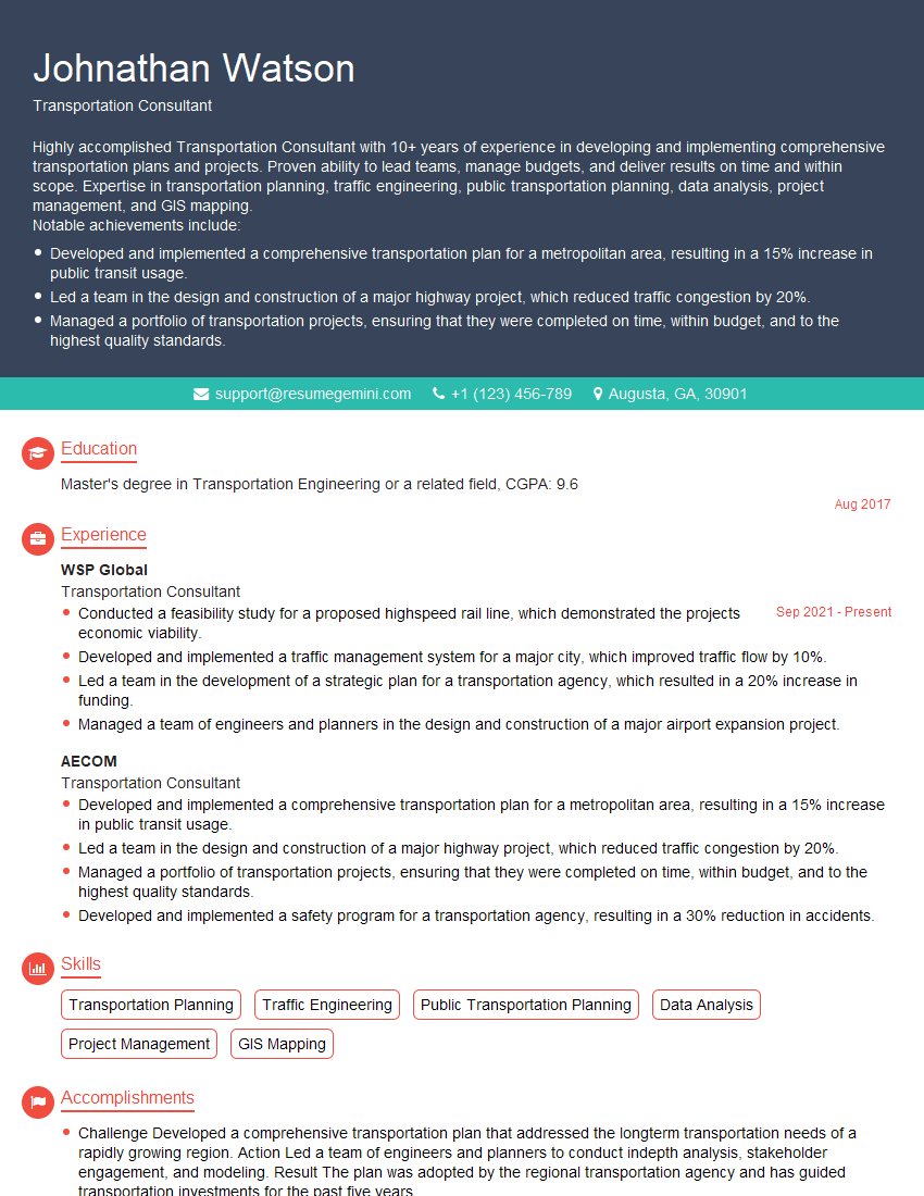
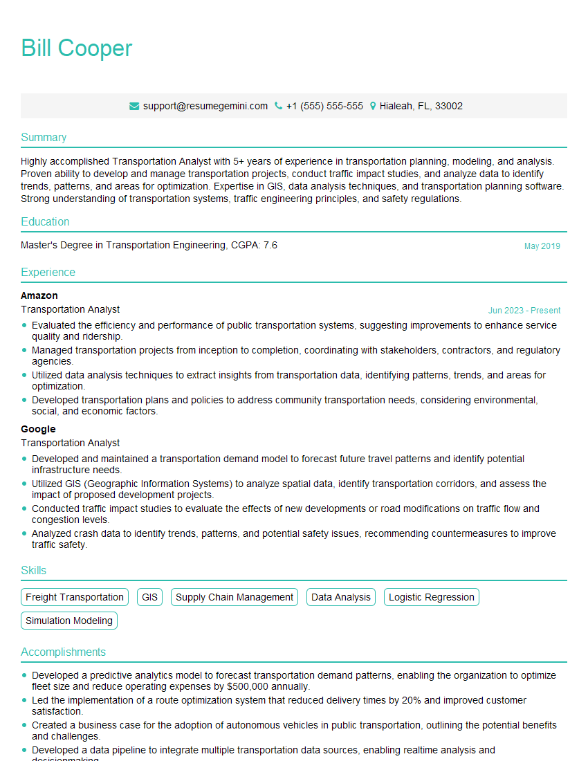
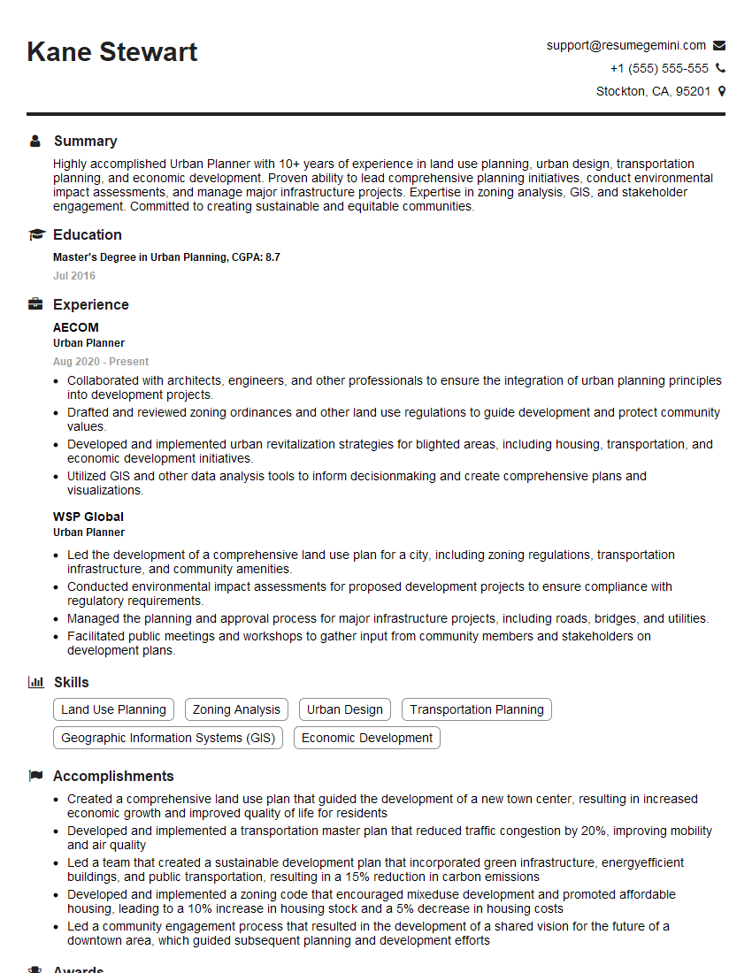
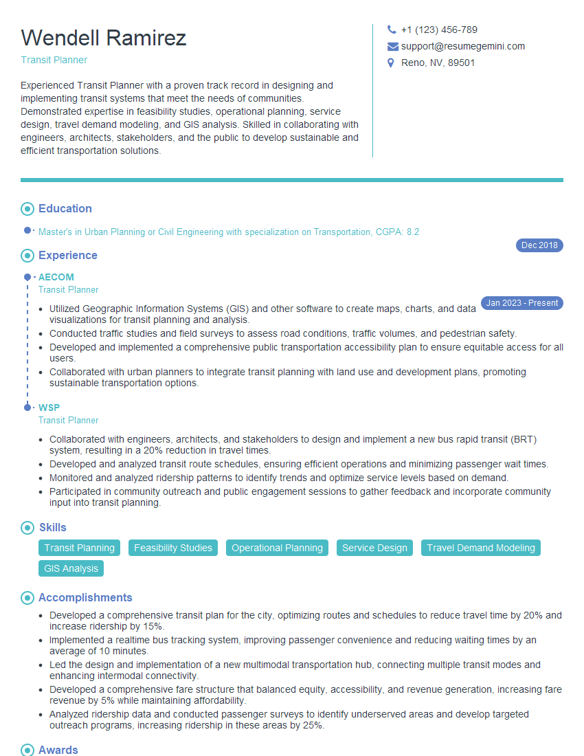
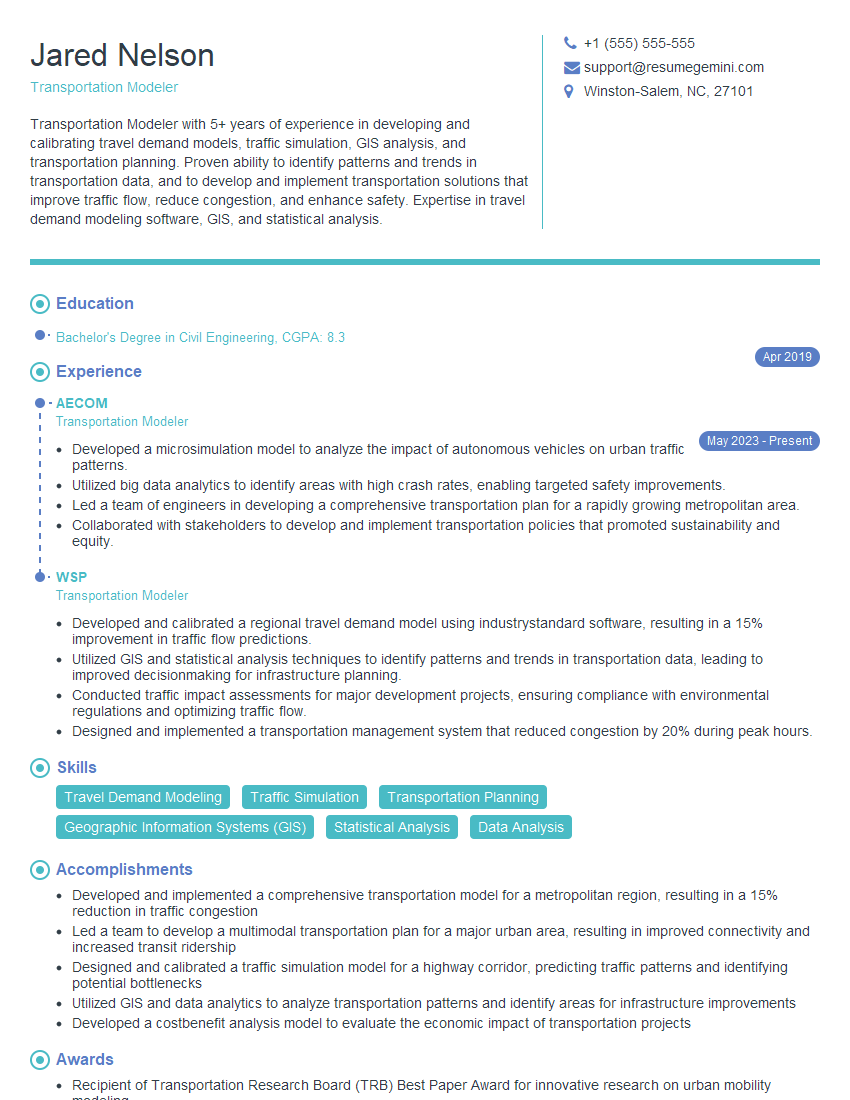
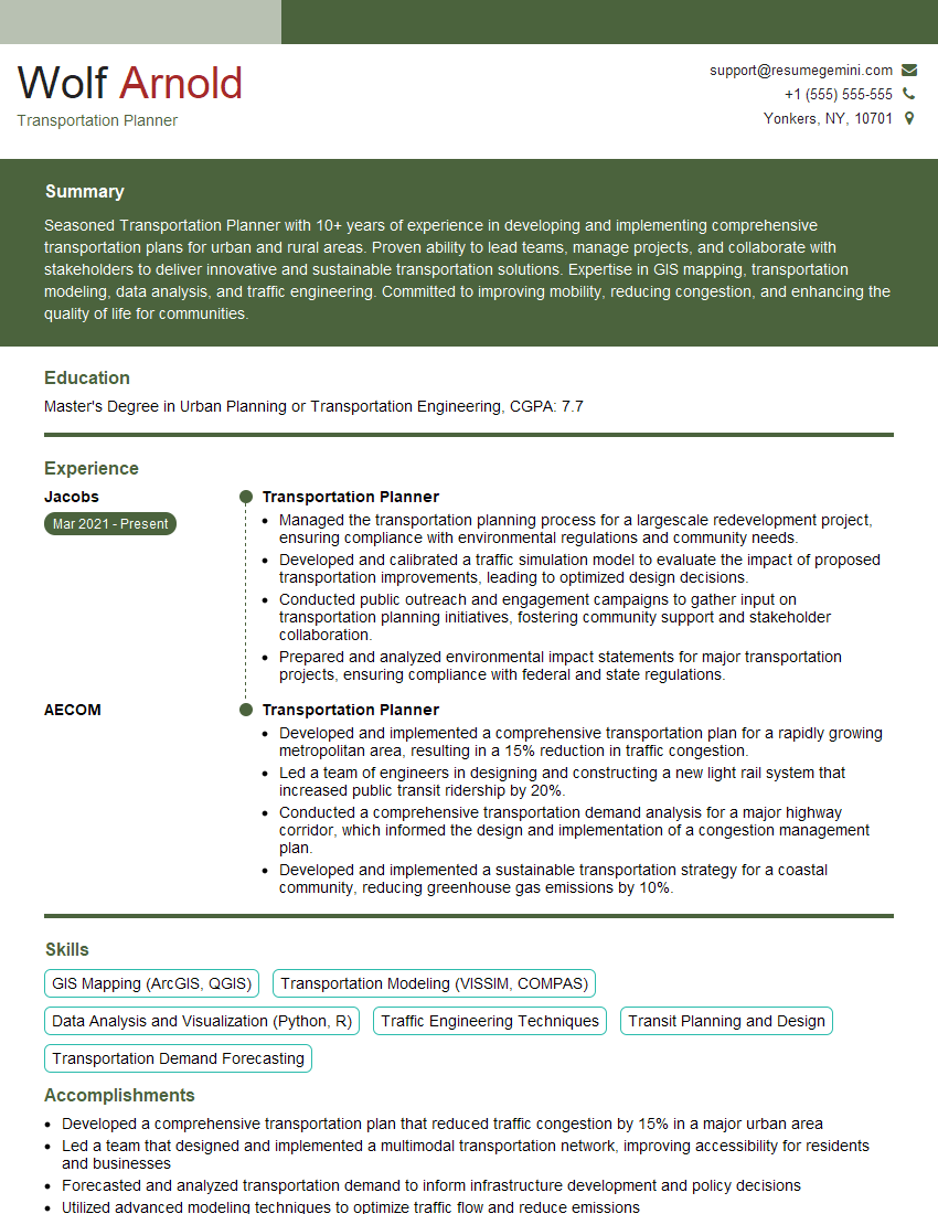
Mastering Transportation Demand Forecasting opens doors to exciting career opportunities in urban planning, transportation engineering, and consulting. These roles are highly sought after, offering both intellectual stimulation and significant impact on communities. To maximize your chances, a strong, ATS-friendly resume is critical. ResumeGemini can help you craft a compelling resume that highlights your skills and experience effectively. We provide examples of resumes tailored specifically to Transportation Demand Forecasting to guide you in creating a document that truly showcases your potential. Invest in your future; build a resume that gets noticed.


Explore more articles
Users Rating of Our Blogs
Share Your Experience
We value your feedback! Please rate our content and share your thoughts (optional).
What Readers Say About Our Blog
To the interviewgemini.com Webmaster.
Very helpful and content specific questions to help prepare me for my interview!
Thank you
To the interviewgemini.com Webmaster.
This was kind of a unique content I found around the specialized skills. Very helpful questions and good detailed answers.
Very Helpful blog, thank you Interviewgemini team.